

Derivative Interactions and Contact Terms
A derivative acting on a field contributes when that field carries incoming momentum in the site Fourier convention. The vertex is obtained by differentiating the written action with respect to its fields, so identical-field multiplicities and the placement of derivatives must be handled before simplifying with momentum conservation. Integration by parts gives equivalent integrated actions under controlled boundary conditions, but derivatives of time-ordered products can also create local delta-function contact terms. In particular, a Hamiltonian interaction containing time derivatives cannot always be replaced blindly by .
Required background. Momentum-Space Feynman Rules fixes the all-momenta-incoming and Fourier conventions.
Helpful background. Coincident Products and Contact Terms explains why local products need a distributional definition; Local versus Integrated Operator Redundancies separates equality after integration from equality of local insertions.
Momentum factors from declared derivatives
Section titled “Momentum factors from declared derivatives”For
one has
Consider two real fields with
Let be the momenta on the two identical legs and the momentum on , all incoming. The two derivatives give ; multiplication by the in the density and by from gives . The two attachments of the identical fields cancel the , leaving
The result is symmetric under , as it must be. Its mass dimension also matches the original local operator: the two momenta supply the two derivative dimensions.
The same map appears in the chapter’s action-to-rule figure. Here the important row is the derivative branch and its explicit identical-field check.
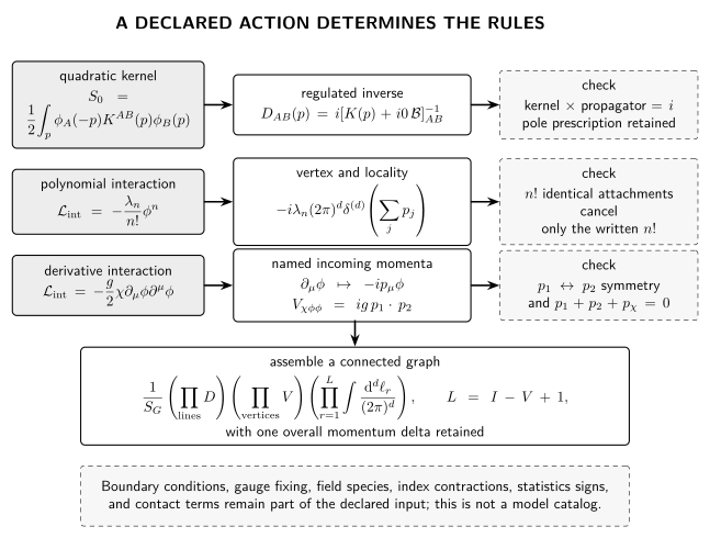
Derivative vertices are obtained from the written action before momentum conservation or on-shell identities are used. The displayed branch yields after the two identical attachments cancel . Quadratic and polynomial branches are included for comparison. Schematic, not to scale.
| Written term | Incoming-momentum numerator | Combinatorial check |
|---|---|---|
| identical attachments cancel | ||
| exchange of the two legs cancels | ||
| for distinct , the derivative belongs only to the leg | ||
| vertex proportional to | vanishes at a momentum-conserving integrated vertex under the stated boundary assumptions |
Integration by parts and total derivatives
Section titled “Integration by parts and total derivatives”Up to a boundary term,
The two forms give the same integrated vertex once all terms are retained and momentum conservation is used. More generally, for , a scalar total-divergence interaction transforms as
where the second expression includes the factor from and any couplings or derivative numerators are contained in . The vertex vanishes against . Schwartz demonstrates this momentum-conservation check for total derivatives in perturbative matrix elements Schwartz 2014, § 7.4, p. 100.
The conclusion has limits. It assumes the boundary term vanishes or is canceled, and it concerns the integrated perturbative vertex. A local operator and that operator plus a total derivative are not pointwise identical. Boundaries, defects, operator insertions carrying momentum, and topological sectors can make the discarded term consequential.
Equations of motion require similar care. Replacing by is valid only in an appropriate on-shell matrix element or after a controlled field redefinition. It is not an algebraic identity inside an off-shell correlator: acting the inverse kinetic operator on a time-ordered propagator produces a contact distribution.
Time ordering creates contact terms
Section titled “Time ordering creates contact terms”For the canonical scalar, equal-time commutation gives
Differentiating a time-ordered product twice therefore yields
Combining spatial derivatives and the free equation of motion gives the distributional inverse relation
The delta term is not an optional correction: it is what makes the inverse of the kinetic operator with the declared normalization. Consequently, moving derivatives through or using the equations of motion inside a correlator can create local contact contributions.
Why time-derivative interactions need special care
Section titled “Why time-derivative interactions need special care”For interactions without time derivatives, canonical momenta are unchanged and . With time derivatives, the relation between velocities and canonical momenta changes; the Legendre transform can generate additional interaction terms. An operator derivation must include them, together with contact terms from differentiated time ordering.
A one-field toy model makes the issue explicit. If the time-derivative part of the Lagrangian is
then and the corresponding Hamiltonian term is
The first interaction term agrees with only after the lowest-order relation is used, and the order- contact interaction has no counterpart in that naive replacement. In a covariant Lagrangian calculation, differentiated time ordering and the momentum-integration measure reorganize the same local information.
The Lagrangian path integral often repackages these contributions into covariant rules, but only after the momentum variables and any field-dependent measure have been handled correctly. Weinberg derives the Lagrangian path integral from the Hamiltonian and states the conditions under which the ordinary Lagrangian appears Weinberg 1995, § 9.3, pp. 389–394; his subsequent rule derivation shows how differentiated contractions give momentum numerators Weinberg 1995, § 9.4, pp. 395–398. Srednicki gives an explicit warning that time derivatives require a conjugate-momentum source in the operator treatment Srednicki 2007, § 9, p. 82.
Thus the safe procedure is not “replace every derivative by momentum” in isolation. It is:
- declare whether the derivation is canonical or Lagrangian;
- derive canonical momenta if time derivatives occur;
- keep the contact terms implied by ordered distributions;
- include the measure or determinant produced when momenta are integrated out; and
- compare a simple correlator or amplitude between the two formulations.
Local contact vertices
Section titled “Local contact vertices”A local monomial such as produces a four-leg contact vertex even though it contains no propagator. Derivative contact vertices are equally local: their polynomial momentum numerator does not turn them into exchange diagrams. Conversely, canceling a propagator denominator with a factor such as can collapse part of a graph to a contact distribution. The distinction is analytic: a genuine exchange contribution has an uncanceled propagator pole, while a contact term is polynomial in momenta at that stage.
This diagnostic is useful under integration by parts and field redefinitions. Different action representatives can redistribute polynomial contact pieces and exchange numerators while leaving a properly defined on-shell amplitude unchanged. Off-shell Green functions need not be identical.
Common pitfalls
Section titled “Common pitfalls”Assigning the derivative momentum to the wrong leg. A derivative acts on its named field. Momentum conservation may rewrite the result only after the unsimplified vertex has been derived.
Using equations of motion inside a time-ordered product without contact terms. The inverse kinetic operator acting on yields , not zero.
Assuming with time derivatives. The canonical momentum and Legendre transform change. Derive them or use a justified Lagrangian path-integral formulation.
Check your understanding
Section titled “Check your understanding”Derive the vertex above, integrate the interaction by parts, and derive it again without imposing on-shell equations.
Solution
The original term gives . After integration by parts, differentiate which of the two identical fields occupies each slot. The term contributes
while contributes
Using , their sum is
with no use of .
Where to continue
Section titled “Where to continue”- Separate contact and pole contributions in amplitudes: Tree Amplitudes and Gauge Consistency applies the analytic distinction to complete trees.
- Define coincident insertions: Coincident Products and Contact Terms treats products that are singular before renormalization.
- Organize operator redundancies only after the observable is fixed: Renormalization and Effective Field Theory treats field redefinitions and operator-basis reduction.
References
Section titled “References”- Schwartz, Matthew D. Quantum Field Theory and the Standard Model. Cambridge: Cambridge University Press, 2014. DOI.
- Srednicki, Mark. Quantum Field Theory. Cambridge: Cambridge University Press, 2007. DOI.
- Weinberg, Steven. The Quantum Theory of Fields, Volume I: Foundations. Cambridge: Cambridge University Press, 1995. First edition; 2005 paperback, 2012 printing consulted. DOI.
Original QFT.org content:CC BY 4.0, unless an item supplies different terms. Third-party material retains its own terms.