Partial-Wave Unitarity

Angular-momentum projection diagonalizes two-body rotational kinematics. With a declared normalization, $S$-matrix unitarity then becomes a separate circle condition for each elastic partial wave and an inequality when inelastic channels open. The circle’s radius, center, and threshold powers are normalization-dependent; the eigenvalue $S_\ell$ is the invariant object.

Required background. S-Matrix Unitarity supplies the operator relation. Relativistic Scattering Kinematics supplies center-of-mass variables and thresholds.

Fix the four-dimensional scalar normalization

For equal-mass spinless $2\to2$ scattering, let

$$\begin{aligned} z&=\cos\theta,\\ \rho(s)&=\sqrt{1-\frac{4m^2}{s}} =\frac{2p_{\mathrm{cm}}}{\sqrt{s}}. \end{aligned}$$

and expand

$$\mathcal M(s,z) =16\pi\sum_{\ell=0}^{\infty}(2\ell+1)a_\ell(s)P_\ell(z).$$

Orthogonality gives

$$a_\ell(s) =\frac{1}{32\pi}\int_{-1}^{1}\mathrm dz\, P_\ell(z)\mathcal M(s,z).$$

The coefficients are fixed rather than guessed: multiplying the expansion by $P_L(z)$ and using

$$\int_{-1}^{1}\mathrm dz\,P_L(z)P_\ell(z) =\frac{2}{2\ell+1}\delta_{L\ell}$$

leaves $32\pi a_L$. Projecting the two-body part of the unitarity state sum with the same identity makes different $\ell$ values orthogonal and yields $\operatorname{Im}a_\ell=\rho|a_\ell|^2$ when no other channel is open.

Define

$$S_\ell(s)=1+2i\rho(s)a_\ell(s).$$

Below the first inelastic threshold, unitarity requires

$$\begin{aligned} |S_\ell|&=1, &S_\ell&=e^{2i\delta_\ell},\\ a_\ell&=\frac{e^{i\delta_\ell}\sin\delta_\ell}{\rho}. \end{aligned}$$

Consequently,

$$\operatorname{Im}a_\ell =\rho|a_\ell|^2.$$

Weinberg derives the relativistic partial-wave decomposition, phase shifts, and threshold behavior in Weinberg 1995, § 3.7, printed pp. 151–159.

The Argand circle and inelastic interior

Introduce the dimensionless amplitude $b_\ell=\rho a_\ell$. In the elastic region,

$$(\operatorname{Re}b_\ell)^2 +\left(\operatorname{Im}b_\ell-\frac12\right)^2 =\frac14.$$

When additional channels open, write

$$S_\ell=\eta_\ell e^{2i\delta_\ell}, \qquad 0\le\eta_\ell\le1.$$

Then

$$\operatorname{Im}b_\ell-|b_\ell|^2 =\frac{1-\eta_\ell^2}{4}\ge0,$$

so $b_\ell$ lies inside the elastic circle. The distance of $S_\ell$ from the unit circle, not a change of plotting convention, measures lost elastic probability. The same diagonal-channel parametrization and its multichannel interpretation are stated in Particle Data Group 2025, review 50, § 50.1.3, printed pp. 8–9, PDF.

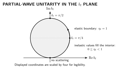
For $b_\ell=\rho a_\ell=(S_\ell-1)/(2i)$, elastic unitarity is the circle $(\operatorname{Re}b_\ell)^2+(\operatorname{Im}b_\ell-1/2)^2=1/4$; the full range $0\le\eta_\ell<1$ fills the interior disk, rather than a distinguished inner circle or universal inward trajectory. The plot is dimensionless and schematic; any energy-dependent path inside the disk is model dependent.

The equivalent semantic data are:

Regime	$S_\ell$	$b_\ell$ constraint
No scattering	$1$	$0$
Elastic	$e^{2i\delta_\ell}$	On the circle, $b_\ell=e^{i\delta_\ell}\sin\delta_\ell$
Inelastic	$\eta_\ell e^{2i\delta_\ell}$, $0\le\eta_\ell<1$	Inside the circle; deficit $(1-\eta_\ell^2)/4$

With several two-body channels, the scalar $S_\ell$ becomes a matrix $S_\ell^{ab}$ in channel space. Unitarity is $S_\ell^\dagger S_\ell=1$ when all open channels in that sector are retained. Diagonalizing this matrix gives eigenphases on the unit circle; looking only at one elastic entry gives $|S_\ell^{aa}|\le1$, with its deficit supplied by transitions to $b\ne a$. The single-channel $\eta_\ell$ parametrization is therefore a projection of multichannel unitary evolution, not a new source of nonunitarity.

For identical particles, form normalized symmetrized or antisymmetrized two-body states before importing these equations. For identical spinless bosons in a symmetric internal state, only even $\ell$ occur. One may integrate the full labeled sphere with exactly one final-state factor $1/2!$, or one representative half-sphere without it. A common normalized-channel convention uses $32\pi$ rather than $16\pi$ in the identical-boson expansion; the corresponding $S_\ell$ relation changes. Preserving the eigenvalue $S_\ell$ is the safe translation check.

Cross sections and threshold scaling

For distinguishable elastic scalars,

$$\sigma_{\mathrm{el}} =\frac{16\pi}{s} \sum_{\ell=0}^{\infty}(2\ell+1)|a_\ell|^2.$$

In the purely elastic region this equals the total cross section obtained from the optical theorem. The maximum contribution of one elastic partial wave follows from $|b_\ell|\le1$:

$$\sigma_\ell\le \frac{4\pi(2\ell+1)}{p_{\mathrm{cm}}^2}.$$

This is a partial-wave bound at fixed energy, not a statement that the full cross section saturates it.

For a short-range interaction and no threshold singularity,

$$\delta_\ell\sim p_{\mathrm{cm}}^{2\ell+1}, \qquad a_\ell\sim p_{\mathrm{cm}}^{2\ell}$$

near threshold. Long-range massless exchange and finely tuned near-threshold states can invalidate this simple scaling. Higher-dimensional harmonic analysis, conformal partial waves, and phenomenological coupled-channel fits use related ideas but different bases and normalizations. Continue to resonance poles and sheets for the analytic meaning of a partial-wave pole; a fitted Argand trajectory alone does not turn an unstable state into an asymptotic particle.

Translate another convention safely

Some sources absorb $\rho$ into the partial amplitude or use $32\pi$ rather than $16\pi$ in the expansion. Do not compare their circles by eye. Compute $S_\ell$ in each convention and demand the same eigenvalue. The phase shift, inelasticity, pole positions, and partial cross section then provide convention-independent checks.

Check your understanding

Starting from $S_\ell=1+2ib_\ell$, impose $|S_\ell|=1$ and complete the square to recover the Argand circle. Then set $S_\ell=\eta e^{2i\delta}$ and derive the inelastic deficit. If your result places $\eta<1$ outside the circle, a sign or normalization is wrong.

Solution

Writing $b=x+iy$, the equation $|1+2ib|^2=(1-2y)^2+4x^2=1$ becomes $x^2+(y-1/2)^2=1/4$. More generally, $|1+2ib|^2=\eta^2$ gives

$$y-(x^2+y^2)=\frac{1-\eta^2}{4}\ge0,$$

so every $0\le\eta<1$ lies in the disk. For fixed $\eta$, varying $\delta$ traces a circle of radius $\eta/2$ centered at $i/2$; allowing the full inelasticity range fills the disk.

References

• Particle Data Group. “Resonances.” In Review of Particle Physics, 2025 Update, review 50, § 50.1.3, printed pp. 8–9. Official PDF.
• Weinberg, Steven. The Quantum Theory of Fields, Volume I: Foundations. Cambridge University Press, 1995, § 3.7, printed pp. 151–159. doi:10.1017/CBO9781139644167.