Soft and Collinear Singularities

Massless propagators become singular in two universal boundary regions of momentum space: a radiated momentum can lose all of its energy, or two null momenta can become parallel. In either case a normally hard internal line is driven on shell. The resulting soft and collinear enhancements overlap, occur in both real and virtual corrections, and must be diagnosed before one can state what cancels or factorizes.

Required background. Anatomy of a Loop Integral supplies loop measures, pole prescriptions, and ultraviolet versus infrared poles. Massless Scalars, Zero Modes, and Infrared Limits explains why the massless limit is not automatically continuous at zero momentum.

Helpful background. Landau Equations and Physical Singularities gives the general pinch-surface criterion used here in its simplest form.

One denominator, two singular limits

Let a massless particle of momentum $p$ emit a massless quantum of momentum $k$. With $p^2=k^2=0$, the adjacent propagator has

$$\begin{aligned} (p+k)^2+i0 &=2p\cdot k+i0\\ &=2E\omega(1-\cos\theta)+i0, \end{aligned}$$

where $E=p^0$, $\omega=k^0$, and $\theta$ is their opening angle. It approaches zero when either

$$\omega\to0 \quad\text{(soft)}, \qquad \theta\to0 \quad\text{(collinear)}.$$

The phase-space measure supplies $\omega\,\mathrm d\omega$ and $\mathrm d\theta^2$ near four dimensions, while the squared emission factor supplies the compensating inverse powers. At leading-logarithmic accuracy the doubly singular part therefore has the schematic form

$$\mathrm d\mathcal P_{\mathrm{sing}} \sim \frac{\alpha C}{\pi} \frac{\mathrm d\omega}{\omega}\, \frac{\mathrm d\theta^2}{\theta^2}.$$

$C$ is the charge or color factor and the omitted finite coefficient depends on the splitting channel and conventions. The endpoint powers, rather than a single coefficient valid in both limits, are the universal feature at this stage. Schwartz derives the soft and collinear phase-space limits and their overlap in Schwartz 2014, § 20.1, printed pp. 356–364.

The geometry is easiest to inspect in logarithmic coordinates. Moving right decreases the emitted energy, moving upward decreases the angle, and the upper-right corner is counted by both approximations.

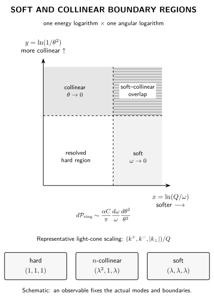
Soft and collinear boundary regions of massless phase space. The logarithmic area generates $\mathrm d\omega/\omega$ and $\mathrm d\theta^2/\theta^2$ enhancements, while the listed light-cone scalings give one representative leading-power organization. The diagram is schematic, not a quantitative phase-space boundary.

Light-cone scaling separates the regions

Choose null vectors $n$ and $\bar n$ with $n\cdot\bar n=2$, and decompose

$$k^\mu=\frac{\bar n\cdot k}{2}n^\mu +\frac{n\cdot k}{2}\bar n^\mu+k_\perp^\mu.$$

For a jet along $n$, a useful representative scaling is

$$\begin{array}{c|c|c} \text{region} & (n\cdot k,\,\bar n\cdot k,\,k_\perp) & k^2 \\ \hline \text{hard} & Q(1,1,1) & Q^2 \\ n\text{-collinear} & Q(\lambda^2,1,\lambda) & Q^2\lambda^2 \\ \text{soft} & Q(\lambda,\lambda,\lambda) & Q^2\lambda^2 \end{array}$$

with $\lambda\ll1$. These entries encode component sizes, including the magnitude of the transverse component; $k_\perp^2<0$ in the site metric. Different observables can require ultrasoft or other scalings, so “soft” is not a regulator-independent numerical assignment. The method of regions is to expand the integrand according to each relevant scaling, integrate the expanded expression over its prescribed domain, and subtract overlaps.

Soft and collinear scalings sit inside a broader loop-momentum diagnostic. The following figure is useful here because it separates homogeneous scaling from the additional contour-pinch question; inspect especially that a collinear momentum can retain a hard component while its virtuality is small.

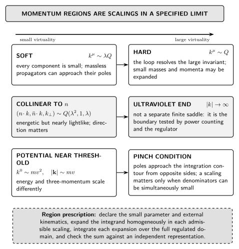
Momentum regions are homogeneous scalings relative to a declared hierarchy, not universal contributions to every integral. This page uses only the soft and collinear entries; the potential scaling belongs to a nonrelativistic threshold, and any claimed singularity still requires the appropriate pinch. The diagram is schematic and not to scale.

Becher, Broggio, and Ferroglia develop this scale analysis in their SCET introduction, arXiv PDF §§ 2 and 4.3, printed pp. 4–8 and 34–37.

Equal virtuality does not mean identical physics: a collinear momentum has a large rapidity because one light-cone component remains order $Q$, whereas a soft momentum has balanced components. This distinction is the source of some rapidity divergences.

Pinches, real emission, and virtual loops

A denominator-level example shows both the power counting and the contour qualification. Let $p_1=Qn/2$ and $p_2=Q\bar n/2$, with $p_1^2=p_2^2=0$ and $2p_1\cdot p_2=Q^2$, and consider

$$I=\mu^{2\epsilon}\int\frac{\mathrm d^{4-2\epsilon}k} {(2\pi)^{4-2\epsilon}}\frac{1}{D_1D_2D_3},$$

where

$$D_1=k^2+i0, \qquad D_2=(p_1-k)^2+i0, \qquad D_3=(p_2+k)^2+i0.$$

Uniform soft scaling $k\sim Q(\eta,\eta,\eta)$ gives

$$\mathrm d^d k\sim Q^d\eta^d, \qquad (D_1,D_2,D_3)\sim Q^2(\eta^2,\eta,\eta),$$

whereas $n$-collinear scaling gives

$$\mathrm d^d k\sim Q^d\lambda^d, \qquad (D_1,D_2,D_3)\sim Q^2(\lambda^2,\lambda^2,1).$$

Both regions therefore scale as the small parameter to the power $d-4$ and are logarithmic at $d=4$. This is only a candidate degree: a numerator zero, Ward identity, or sum over graphs can remove the leading term.

The Landau condition makes the contour statement concrete. On the collinear surface $k=xp_1$ with $0<x<1$, $D_1=D_2=0$ and $D_3$ stays hard. The stationarity equations admit

$$\alpha_3=0, \qquad x\alpha_1=(1-x)\alpha_2, \qquad \alpha_1,\alpha_2>0.$$

This is a physical-sheet pinch candidate for the common $+i0$ prescription. At the soft endpoint $k=0$, all three denominators vanish and a degenerate solution has $\alpha_1>0$, $\alpha_2=\alpha_3=0$. The example establishes where the scalar denominator skeleton can pinch, not the coefficient of a gauge-invariant amplitude. The corresponding massless pinch surfaces and their power counting are reviewed in Agarwal et al. 2023, § 3.1.4, printed pp. 61–62, and § 3.2.2, printed pp. 64–66, PDF.

More generally, a small denominator is physically singular only if the integration contour cannot be deformed away. In a virtual graph, the $i0$ prescriptions of several propagators may trap the energy contour as the relevant lines simultaneously approach their mass shells. In a real correction, the emitted line is already on shell and the same boundary appears directly in phase space. Thus a virtual infrared pole and an unresolved real-emission pole are two sides of the same long-distance kinematics, but they do not cancel until the observable sums the corresponding degenerate configurations.

Dimensional regularization with $d=4-2\epsilon$ often represents both boundaries by $1/\epsilon_{\mathrm{IR}}$ poles. A mass $m$ instead changes the small-angle denominator to

$$2p\cdot k\simeq E\omega \left(\theta^2+\frac{m^2}{E^2}\right),$$

so it cuts off a collinear logarithm at $\theta\sim m/E$ but leaves the $\omega\to0$ soft limit. An energy resolution regulates the real soft integral physically; an auxiliary photon or gluon mass may regulate it algebraically, but in a non-Abelian gauge theory such a mass generally violates gauge symmetry unless introduced within a consistent construction.

A scaleless integral vanishes in dimensional regularization because its UV and IR poles cancel in the regulated expression. It must not be read as evidence that the infrared region was absent. The separation into individual soft and collinear functions is likewise regulator- and subtraction-scheme dependent; only their properly combined observable is scheme independent.

What universality does and does not say

The leading singular terms depend only on the external charges, directions, and spins through universal soft currents and splitting amplitudes. Finite terms, recoil, spin correlations beyond the leading approximation, and power-suppressed contributions remain process dependent. A mass removes a strict collinear divergence but can leave a large logarithm $\ln(Q/m)$, and confinement prevents isolated colored external states from being observables.

This diagnosis does not itself prove cancellation or factorization. It tells us which regions a proof must reproduce, which overlaps it must subtract, and which physical resolution enters the answer.

Exercises

1. Power-count the triangle denominator skeleton in the uniform soft and $n$-collinear regions. Show that both candidates are logarithmic in four dimensions.

   Solution

   The soft measure and denominators scale as $\eta^d$ and $\eta^4$; the collinear measure and denominators scale as $\lambda^d$ and $\lambda^4$. Each ratio is therefore the small parameter to the power $d-4$. A numerator or gauge-invariant graph sum can still suppress the candidate.

2. Repeat the adjacent-propagator analysis for a hard particle of mass $m$ and velocity $v$. Which boundary survives at fixed $m/E$?

   Solution

   The denominator is proportional to $E\omega(1-v\cos\theta)$. At $\theta=0$, $1-v>0$ for fixed nonzero $m/E$, so the strict collinear divergence is removed. The factor still vanishes as $\omega\to0$, so the soft boundary remains.

References

• Agarwal, Neelima, Lorenzo Magnea, Chiara Signorile-Signorile, and Anurag Tripathi. “The Infrared Structure of Perturbative Gauge Theories.” Physics Reports 994 (2023): 1–120, esp. §§ 3.1.4 and 3.2.2. doi:10.1016/j.physrep.2022.10.001. Open PDF.
• Becher, Thomas, Alessandro Broggio, and Andrea Ferroglia. Introduction to Soft-Collinear Effective Theory. Lecture Notes in Physics 896. Springer, 2015, §§ 2 and 4.3, pp. 7–12 and 35–38. doi:10.1007/978-3-319-14848-9. Open PDF.
• Schwartz, Matthew D. Quantum Field Theory and the Standard Model. Cambridge University Press, 2014, § 20.1, printed pp. 356–364. doi:10.1017/9781139540940.