EFT Positivity and UV Consistency

EFT positivity is applied to on-shell amplitude coefficients, not to a basis-dependent Wilson coefficient by inspection. A reliable exclusion first fixes the elastic state and completion assumptions, removes light poles and cuts consistently, extracts a renormalization-scale-independent amplitude combination, and then compares its uncertainty interval with the relevant dispersive inequality.

Required background. Forward-limit positivity bounds supplies the basic conditional theorem. Helpful background. Beyond-forward positivity supplies mixed-derivative and improved constraints.

From an EFT amplitude to a dispersive coefficient

Start with a systematically truncated EFT as described in Effective Field Theory as a Controlled Expansion. For a chosen elastic process, calculate the renormalized on-shell amplitude and decompose it as

$$\begin{aligned} A_{\mathrm{EFT}}(s,t;\mu) ={}&A_{\mathrm{poles}}+A_{\mathrm{light\ nonanalytic}} +A_{\mathrm{local}}\\ &+A_{\mathrm{ref}}\, O\!\left[\left(\frac{Q}{\Lambda}\right)^{p_{\mathrm{next}}}\right]. \end{aligned}$$

Here $Q$ denotes the low-energy scale, $A_{\mathrm{ref}}$ supplies the amplitude normalization, and $p_{\mathrm{next}}$ is the first omitted power in the declared power counting; it is not automatically the next operator dimension.

Remove only the poles specified by the dispersion relation and define a crossing eigenamplitude. In the identical-scalar benchmark,

$$v=s-2m^2+\frac{t}{2}, \qquad B(v,t)=B(-v,t).$$

The forward coefficient tested by the first bound is

$$C_2^{\mathrm{phys}} =\frac{1}{2}\left.\partial_v^2B(v,0)\right|_{v=0}.$$

At loop level it has the form

$$C_2^{\mathrm{phys}} =C_2^{\mathrm{local}}(\mu)+C_2^{\mathrm{light}}(\mu), \qquad \mu\frac{\mathrm d}{\mathrm d\mu}C_2^{\mathrm{phys}}=0 \quad\text{through the calculated order}.$$

The two terms separately depend on scheme and scale; their physical sum does not, while a truncated result retains dependence of the first omitted order. A field redefinition can also move coefficients among operators while leaving $C_2^{\mathrm{phys}}$ unchanged. This is why the sign of one Lagrangian coefficient is meaningful only after its amplitude map and approximation order are declared.

For a gapped completion satisfying the forward hypotheses,

$$C_2^{\mathrm{phys}} =\frac{2}{\pi}\int_{\nu_0}^{\infty} \frac{\rho(\nu)}{\nu^3}\,\mathrm d\nu\ge0.$$

It is strict when the selected state has nonzero absorptive weight at finite energy. The original scalar EFT obstruction and its dependence on a standard analytic UV completion are explicit in Adams et al. 2006, § 2, pp. 3–4, and § 4, pp. 14–19, PDF.

A reproducible application workflow

1. Specify the amplitude. Give external species, polarizations, internal-state superpositions, normalization, and the crossing eigenchannel.
2. State the completion class. Record Lorentz invariance, unitarity, real analyticity, locality or polynomial boundedness, mass gap, and the assumed number of subtractions.
3. Choose a safe point. Put the subtraction point below all cuts and away from stable poles. Verify that it lies inside the fixed-$t$ analytic domain.
4. Calculate to one order. Include local operators, exchange graphs, counterterms, and light loops through a consistent EFT and coupling order.
5. Subtract known infrared data. Remove stable poles exactly. If using an improved bound, subtract the calculable low-energy absorptive integral in the same convention.
6. Extract amplitude coefficients. Differentiate the pole-subtracted amplitude and translate the result to basis-invariant Wilson-coefficient combinations where possible.
7. Apply the correct inequality. Use the forward, beyond-forward, or full-crossing kernel actually proved for the chosen states.
8. Propagate uncertainty. Include truncation, perturbative, input, numerical, and subtraction uncertainties before declaring exclusion.

The pole-subtracted scalar implementation and its derivative hierarchy are given in de Rham et al. 2017, pp. 1–4, PDF.

A one-loop matching example

For the heavy-scalar model on the forward page, the full-theory coefficient is

$$C_2^{\mathrm{full}} =\frac{\lambda^2}{32\pi^2} \int_0^1\mathrm dx\, \frac{x^2(1-x)^2} {[M^2-2m^2x(1-x)]^2}.$$

At leading order in $m^2/M^2$, match onto

$$X=\frac12\partial_\mu\phi\,\partial^\mu\phi, \qquad \mathcal L_{\mathrm{EFT}}supset\frac{c_X}{M^4}X^2.$$

In the otherwise free light theory, no light loop contributes to this moment at order $\lambda^2$, so matching through dimension eight gives

$$\boxed{c_X(\mu=M)=\frac{\lambda^2}{960\pi^2}>0}.$$

The next term, $6m^2/(7M^2)$ relative to the leading result, belongs to higher-dimensional operators; assigning the exact integral to $c_X$ would hide the EFT truncation. This example also separates the basis-dependent coordinate $c_X$ from the physical moment: here the map is one-to-one at the retained order, but in a general basis several coefficients and light-loop terms contribute to the same $C_2^{\mathrm{phys}}$.

Improved constraints and scale separation

Suppose the EFT predicts the absorptive part up to $\nu_{\mathrm{IR}}$. Then test

$$C_{2,\mathrm{UV}} =C_2^{\mathrm{phys}} -\frac{2}{\pi}\int_{\nu_0}^{\nu_{\mathrm{IR}}} \frac{\rho_{\mathrm{EFT}}(\nu)}{\nu^3}\,\mathrm d\nu\ge0.$$

The inequality is strict only if spectral weight remains above $\nu_{\mathrm{IR}}$. The subtraction isolates that high-energy remainder and can strengthen the constraint, but only when the scale hierarchy

$$\nu_0<\nu_{\mathrm{IR}}\ll\Lambda^2$$

and the perturbative accuracy of $\rho_{\mathrm{EFT}}$ are adequate. Moving $\nu_{\mathrm{IR}}$ changes both terms; a residual dependence larger than the quoted error signals an inconsistent truncation.

At higher order, the coefficients are correlated moments. With $x=\nu^{-2}\in[0,X]$, positive spectral weight generates the normalized region shown below. The figure is a diagnostic for coefficient combinations: a point outside cannot arise from the stated positive measure, while a point inside is not by itself a UV construction.

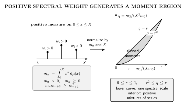
Schematic amplitude-coefficient constraint. After consistent pole and infrared treatment, three successive forward coefficients define moments $m_0,m_1,m_2$ and ratios satisfying $r^2\le q\le r$. The region assumes a compact positive measure and is not sufficient evidence for a UV completion.

EFT operation	Moment-figure counterpart
compute physical derivative combinations	determine $m_0,m_1,m_2$
divide by the threshold scale and $m_0$	form dimensionless $r,q$
test Hankel positivity	require $q\ge r^2$
use the spectral gap	require $q\le r$
include several heavy states	form positive mixtures in the interior

The complete positive-moment constraints are developed in Bellazzini et al. 2021, § I.A–B, pp. 2–5, PDF. Their translation to tree-level Wilson coefficients, and the loop-corrected RG-invariant amplitude quantities that replace those coefficients beyond tree level, are analyzed in Bellazzini et al. 2021, § II.A–B, pp. 6–11, PDF.

Exclusion with uncertainties

Let $P$ be the left-hand side of a positivity inequality, with an estimate $\widehat P$ and conservative total error $\Delta P$. Then:

Result	Defensible statement
$\widehat P-\Delta P>0$	this test is passed at the quoted accuracy
$\widehat P+\Delta P<0$	the EFT point is incompatible with the stated completion class at the quoted accuracy
interval overlaps zero	the calculation is inconclusive

For an EFT truncated after dimension $D$, a schematic truncation estimate is

$$\Delta P_{\mathrm{trunc}} \sim P_{\mathrm{ref}} \left(\frac{Q}{\Lambda}\right)^{D_{\mathrm{next}}-D},$$

but the coefficient multiplying this estimate must reflect the actual power counting. Near cancellations, neglected loop or higher-dimension terms can dominate the quantity being tested.

Interpretation boundaries

Necessary, not sufficient. A passed set of bounds does not construct a UV theory, establish locality, or prove that every higher moment can be completed consistently.

Completion-class dependent. A violation excludes the simultaneous assumptions used in the derivation. It does not show which assumption fails.

Amplitude based. Apparent negativity of an individual Wilson coefficient can disappear after basis translation, crossing projection, or light-loop inclusion.

Not RG replacement. Matching and running determine the coefficient combination entering the amplitude. Positivity constrains the resulting physical combination; it does not calculate its RG evolution.

Massless caution. If a photon, gluon, or graviton produces a forward singularity, use the infrared analysis before applying any forward inequality.

Exercises

A calculation finds $\widehat P=-0.03$, truncation error $0.02$, and loop-scale variation $0.015$. Can it exclude the stated UV-completion class if the two errors are added conservatively?

Check

No. The conservative interval is $-0.03\pm0.035$, which overlaps zero. The result is inconclusive even though the central value is negative.

For EFT construction, matching, and running: Renormalization and Effective Field Theory. For the controlled expansion used here: Effective Field Theory as a Controlled Expansion.

References

• Adams, Allan, Nima Arkani-Hamed, Sergei Dubovsky, Alberto Nicolis, and Riccardo Rattazzi. “Causality, Analyticity and an IR Obstruction to UV Completion.” Journal of High Energy Physics 10 (2006): 014. DOI. Open PDF.
• Bellazzini, Brando, Joan Elias Miró, Riccardo Rattazzi, Marc Riembau, and Francesco Riva. “Positive Moments for Scattering Amplitudes.” Physical Review D 104 (2021): 036006. DOI. Open PDF.
• de Rham, Claudia, Scott Melville, Andrew J. Tolley, and Shuang-Yong Zhou. “Positivity Bounds for Scalar Theories.” Physical Review D 96 (2017): 081702. DOI. Open PDF.