

Foundations of Quantum Field Theory
Quantum field theory is not a single formula or a single quantization recipe. In this volume it is a controlled quantum structure of local fields or observables, states, correlations, dynamics, relativistic spacetime assumptions, and limits. Where a particle interpretation exists, that structure also describes the creation and annihilation of excitations; gauge, topological, thermal, curved-spacetime, and other settings require qualifications supplied by the respective volumes. To say which QFT is being used, one must identify the objects, state, spacetime setting, observables, and any domain, regulator, boundary condition, or limiting prescription that makes its expressions meaningful.
This volume builds that description from one controlled example: the free real scalar field. The same model is followed through canonical quantization, regulated functional integration, spectral analysis, Lorentzian and Euclidean correlators, and structural locality tests. Fermions and spin-one fields then show which parts of the scalar story survive and which require new algebra, constraints, or gauge qualifications. The final chapters explain why an interacting Lagrangian is important data but not, by itself, a complete definition of an interacting continuum theory.
Helpful background. Field Variations and Boundary Terms supplies the variational and boundary-term checks used in action-based formulations. Lorentz Field Representations and Poincaré Particle Representations separates covariant field labels from particle-state representations. Test-Function Spaces, Distributions, Support, and Convergence supplies smearing, support, and distributional convergence, while Fourier Series, Fourier Transforms, and Plancherel Theory supplies the transform and mode-normalization tools used throughout the volume.
The object comes before the calculation
Section titled “The object comes before the calculation”Several objects that are often called “the QFT” are related but not identical:
- A theory specifies the physical content: observables, states, dynamics, spacetime setting, symmetries, and a domain in which its predictions are defined.
- A field is a spacetime-indexed insertion or coordinatization. It need not itself be an observable, and it is not a particle.
- A state assigns expectation values to observables. A vacuum is a state with additional symmetry and energy properties, not a synonym for an empty classical configuration.
- A representation realizes an abstract algebra on a Hilbert space. In QFT, different physically relevant representations need not be unitarily equivalent.
- A particle is a particular kind of state or spectral structure. Particle language can be exact for a free field, asymptotic in a scattering problem, state-dependent in other settings, or unavailable.
- A formulation chooses primitive objects and a method of calculation: canonical operators, functional integrals, Euclidean functions, local observable algebras, or another controlled construction.
The distinction between an observable algebra, a state, and its Hilbert-space representation is especially important in systems with infinitely many degrees of freedom; it prevents one chosen Fock space from being mistaken for universal kinematics. Fewster and Rejzner 2019, arXiv v2 preprint, §§ 2.2–2.3, pp. 5–9, and § 4.1, pp. 13–15, Open PDF give a precise algebraic account of these layers and explain why inequivalent representations occur in QFT. The canonical and functional descriptions developed here remain indispensable, but their agreement is always a statement with hypotheses, not a license to identify every formal expression.
Choose a route by the question
Section titled “Choose a route by the question”| If you want to know… | Start with… | Then continue to… |
|---|---|---|
| What a field, state, observable, representation, or particle is | Quantum Fields, States, and Observables | States, Observables, and Spectra |
| How a local action produces equations and initial data | Classical Local Fields and Actions | Canonical Quantization and the Free Scalar |
| How to quantize the simplest relativistic field | Canonical Quantization and the Free Scalar | Correlators, Sources, and Effective Actions |
| What a path integral actually integrates | Functional Integrals and Free Gaussian Fields | Lorentzian, Euclidean, and In-In Formulations |
| How spinors and anticommuting variables enter | Free Fermion Fields | Structural Principles and Axiom Maps |
| Why photons require constraints and gauge qualifications | Free Spin-One Fields and Constraints | Symmetry and Gauge Structure |
| How sources organize correlators and exact identities | Correlators, Sources, and Effective Actions | Local Operators and Short-Distance Structure |
| How poles, cuts, and spectral weight encode physical content | States, Observables, and Spectra | Perturbative QFT and Scattering |
| Why local products and contact terms need care | Local Operators and Short-Distance Structure | Renormalization and Effective Field Theory |
| Which correlator or contour answers a given physical question | Lorentzian, Euclidean, and In-In Formulations | Thermal and Nonequilibrium QFT when an initial ensemble or nonequilibrium evolution is central |
| Which assumptions support covariance, positivity, locality, spin–statistics, or CPT | Structural Principles and Axiom Maps | Mathematical QFT for theorem-level constructions and comparisons |
| What an interacting Lagrangian does—and does not—define | Interacting QFT: Definitions, Limits, and Handoffs | The construction volume named by the regulator, observable, and limit you need |
Readiness check
Section titled “Readiness check”The volume overview has no hard prerequisite. Use the following routing prompts for the route you intend to follow.
| Capability | Try this inspectable task | A sufficient answer | Unlocks | Repair and return |
|---|---|---|---|---|
| Field variation | Vary without discarding a term. | You obtain a bulk term proportional to and a boundary integral, and you can name data that make the latter vanish or cancel. | Chapters 2–4 | Review Field Variations and Boundary Terms, then return to Chapter 2. |
| Fourier normalization | Starting from one stated Fourier pair, derive the corresponding delta-function identity. | The signs and every factor of agree in the forward transform, inverse transform, and delta distribution. | Modes, propagators, spectra, and functional integrals | Review Fourier Series, Fourier Transforms, and Plancherel Theory, then return to the free scalar. |
| Distributions | Explain what means that the point symbol does not. | You identify the test function, support, linearity, and why coincident products require a separate prescription. | Smearing, causal support, propagators, and local insertions | Review Test-Function Spaces, Distributions, Support, and Convergence, then return to Chapter 1. |
| Relativistic state labels | For and , say which data distinguish a one-particle species and which measure is invariant. | You name mass and spin or helicity, include internal quantum numbers and additional species labels when needed, and recognize up to a declared convention. | Particle states, fermions, vectors, and spectral support | Review Lorentz Field Representations and Poincaré Particle Representations, then return to one-particle states. |
For a broader diagnostic, use Readiness. The compressed QFT refresher serves an experienced returning reader; mathematical foundations for physicists and physical foundations for mathematicians provide longer bridges. In every case, return as soon as the particular task above becomes inspectable; no reader must complete all four repairs before entering the volume.
The free-scalar Rosetta stone
Section titled “The free-scalar Rosetta stone”The recurring comparison begins with one controlled system, not with an unqualified continuum symbol. Take a real scalar of mass on , where is the cubic spatial torus of side , impose periodic spatial boundary conditions, and retain only momenta
The band-limited field has action
Choose the positive-frequency vacuum, represent the canonical commutation relation algebra generated by the finitely many retained modes on its Fock space, and use finite-particle vectors as the common working domain. Then
The vacuum time-ordered two-point function is consequently the finite sum
This formula fixes the mode normalization, state, ordering, and target two-point object together. The oscillator construction and equal-time normalization are developed in Schwartz 2014, §§ 2.2–2.3, pp. 17–26.
For the functional description, also divide a declared Euclidean interval into steps of width , collect the finitely many field values into , and include boundary wave functions that prepare the same canonical state. After Euclidean continuation under the hypotheses stated in Chapter 10, the quadratic form is a positive matrix and
Here the covariance is exactly the inverse of the regulated kernel. If is built from the same finite Trotter product used on the canonical side, the two descriptions match at that discretized level when ordering, normalization, and boundary states agree. Equality with exact canonical time evolution additionally requires the time-step limit; removing the spatial mode cutoff and finite box introduces separate limits. Schwartz 2014, §§ 14.2–14.3, pp. 254–264 derives the time-sliced and Gaussian formulas; Zinn-Justin 2021, § 1.1, pp. 1–3, and §§ 7.1–7.3, pp. 126–130 gives the finite determinant formula, normalized Gaussian, and inverse kernel.
After removing the cutoff and taking the infinite-volume limit for the free model, the continuum two-point function may also be written
This representation assumes a Poincaré-invariant vacuum, positive Hilbert-space metric, the forward-cone spectrum condition, and the regularity needed for the two-point distribution. For the canonically normalized free field, ; interacting scalar theories satisfying those hypotheses can add continuum weight. The intermediate-state derivation and positivity scope appear in Schwartz 2014, § 24.2.1, pp. 467–469.
The following map separates three comparisons that are often compressed into one claim of “equivalence.” Inspect the line styles: each route has its own objects, regulator or limiting stage, and hypotheses.
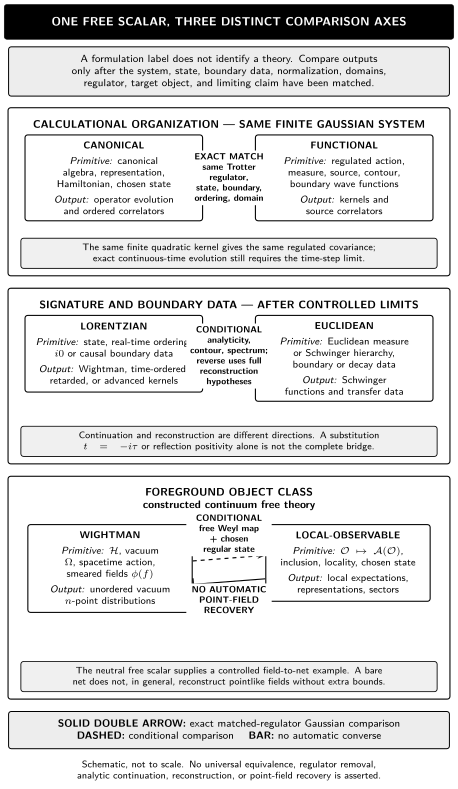
For one free scalar, canonical–functional agreement is exact only for the matched finite Trotter-regulated Gaussian system, while Lorentzian–Euclidean and Wightman–local-observable comparisons carry distinct hypotheses. Solid, dashed, and barred routes mark an exact matched-regulator comparison, a conditional comparison, and no automatic converse; the map is schematic and not to scale.
Original diagram: OpenAI Codex for QFT.org, CC BY 4.0. Editable TikZ source · Sources and reproduction notes.
Read without the graphic: the canonical and functional lanes agree only when the finite system, Trotter kernel, prepared state, boundary data, ordering, normalization, and domains match. Lorentzian continuation and Euclidean reconstruction are different conditional directions, and constructing the neutral free scalar’s Weyl net does not make point-field recovery from a bare local net automatic. The semantic table below lists the data that are held fixed in the regulated comparison and the claims that remain separate.
| Rosetta entry | Matched reference data | Appearance across descriptions | What may change or must still be proved |
|---|---|---|---|
| System | Massive real scalar on ℝ × 𝕋L3, with 𝕋L3 the cubic torus of side L | The finite canonical and functional descriptions use the same regulated system. Later Lorentzian, Euclidean, spectral, and structural statements concern the corresponding family only after the limits required by each statement are controlled. | Massless, complex, spinor, and vector fields require separate checks. |
| State and boundary data | Positive-frequency Fock vacuum, periodic space, and matched time-boundary wave functions | Canonical vacuum expectations, Lorentzian boundary values, and the Euclidean covariance are compared for the same prepared Gaussian state. | Thermal, in–in, scattering, and curved-spacetime states are different data. |
| Algebra and domain | Canonical commutation relation algebra for finitely many modes, represented on Fock space with the finite-particle subspace as a common invariant domain | Canonical operators and finite Gaussian variables provide two regulated descriptions; the spectral and structural statements use the resulting two-point object. | Continuum fields are distributions and need domain and product control. |
| Fourier and mode normalization | L−3/2 modes, 1/√(2ωn), and [an,ar†] = δnr | The same normalization fixes the canonical commutator, finite-volume propagator, and source covariance; after the continuum limit, retaining canonical normalization fixes the free spectral pole weight. | Another Fourier convention is equivalent only after every measure, delta function, mode, operator, and state normalization is translated together. |
| Regulator and limits | Finite spatial mode set and an M-step Trotter discretization on a declared Euclidean time interval | The finite-mode canonical sums and the covariance KM,N−1 of the finite Gaussian discretization are exact within their respective regulated constructions. They agree only when KM,N is built from the same M-step Trotter kernel, not from exact-time evolution. | No time-continuum, cutoff-removal, infinite-volume, or zero-mass limit is automatic. |
| Target two-point object | Vacuum time-ordered two-point function and its Euclidean covariance | Canonical ordering, Gaussian source differentiation, spectral support, and continuation are compared for this declared two-point object. A correlator is not automatically a directly measured observable. | Responses, in–in expectations, unordered correlators, and scattering amplitudes use different orderings, contours, or asymptotic data. |
| Strength of comparison | Exact Gaussian identities and equality with the same Trotterized kernel | The finite canonical and functional descriptions agree after the system, state, boundary data, normalization, regulator, and target two-point object are matched. | Exact-time evolution, regulator removal, analytic continuation, reconstruction, and framework equivalence remain separate conditional claims. |
The restriction avoids a zero-frequency mode in this reference system; the massless page later treats the finite-volume and infrared obstruction explicitly. At finite and , exact checks are the discrete dispersion relation, the truncated equal-time delta, positivity of the oscillator Hamiltonian, and inversion of . Causal support of the continuum Pauli–Jordan commutator and retarded or advanced kernels, exact Poincaré covariance, the continuum delta, and the Källén–Lehmann form are checks only after the relevant time, cutoff, and volume limits have been controlled. A finite cubic cutoff itself is not Lorentz invariant and need not preserve exact continuum microcausality.
Original table: QFT.org editorial project; original semantic table drafted with OpenAI Codex at the user’s direction. CC BY 4.0. Editable HTML table · Sources and reuse notes.
Twelve chapters
Section titled “Twelve chapters”The order below is the sidebar order, not a claim that every reader must traverse every chapter. “Enter” names the preparation for the chapter’s main calculation; individual orientation leaves may be available earlier.
| Chapter and durable purpose | Enter and representative question | Observable exit | Stopping boundary, likely blocker, and route role |
|---|---|---|---|
| 1. Quantum Fields, States, and Observables separates theories, formulations, fields, observables, states, representations, particles, smearing, and locality. | Enter directly through the formulation map, one-particle states, or distributions. Ask whether a free scalar field is a particle, an observable, or an interpolating operator. | Normalize one- and multiparticle states and state a qualified spacelike-locality test. | Stops before GNS and local-net proofs, LSZ, and gauge-invariant construction. Blocker: identifying a field, particle, and observable. Core conceptual and rigorous-doorway role. |
| 2. Classical Local Fields and Actions supplies the local action, boundary, Hamiltonian, and free-current data needed for quantization. | Enter with elementary mechanics and integration by parts. Vary the scalar action while keeping its boundary term. | Derive Euler–Lagrange equations and canonical data with dimensions, signs, and allowed variations explicit. | Stops before general symplectic reduction, gauge generators, and curved-spacetime stress tensors. Blocker: silently discarding boundary terms. Core derivation role. |
| 3. Canonical Quantization and the Free Scalar constructs the first complete free-field model and its propagator taxonomy. | Enter the main chain from the scalar action and Klein–Gordon modes; canonical-bracket orientation is also a direct entry. Check one mode normalization against the equal-time commutator. | Build the algebra, Fock representation, vacuum, particles, propagators, and Schrödinger wave functional, naming each representation-dependent choice. | Stops before interacting renormalization and curved-spacetime particle notions. Blocker: mixing algebra, representation, state, and particle interpretation; massless zero modes need their own page. Core canonical and normalization role. |
| 4. Functional Integrals and Free Gaussian Fields starts with finite variables or a regulator and only then introduces continuum notation. | Enter through the regulated bosonic measure after the action principle; Gaussian sources also require Klein–Gordon modes. Time slicing additionally requires the Schrödinger wave functional, and the canonical–functional capstone requires time slicing, Gaussian sources, and the quantized scalar. | Derive the finite Gaussian source functional, covariance, determinant ratio, and matched Trotterized canonical kernel. | Stops before a general continuum measure, anomaly theorem, or universal formulation equivalence. Blocker: treating a formal product measure as defined. Core functional and computational-check role. |
| 5. Free Fermion Fields connects Lorentz spinors, plane waves, CAR quantization, propagators, and Grassmann integration. | Enter with one-particle representations and the scalar propagator pattern; the Grassmann leaf also uses the Gaussian-integral logic of Chapter 4. Compare chirality with a Majorana reality condition. | Quantize Dirac, Weyl, and Majorana free fields while translating gamma, adjoint, spin-sum, and Berezin conventions. | Stops before Yukawa and gauge dynamics, anomalies, and Standard Model representations. Blocker: identifying negative frequency with negative physical energy or basis-dependent reality with a Majorana condition. Field-species depth role. |
| 6. Free Spin-One Fields and Constraints uses Proca and Maxwell fields to expose constraints, auxiliary covariant variables, and physical polarization counting. | Enter from classical Hamiltonian data and Lorentz representations. Compare the three massive Proca modes with the two physical photon modes. | Count physical modes and distinguish physical-mode from covariant auxiliary-space quantization. | Stops before general constrained reduction, BRST/BV, and interacting gauge theory. Blocker: describing as simply deleting a polarization. Gauge-preparation depth role. |
| 7. Correlators, Sources, and Effective Actions develops , connected , Wick factorization, , and Schwinger–Dyson identities. | Enter from the scalar propagators and Gaussian source functional. Derive one field insertion by differentiating a fully declared source convention. | Translate among full, connected, and 1PI objects and check their kernels, normalizations, and factors of . | Stops before diagrammatics, renormalized effective actions, and causal in–in evolution. Blocker: using mnemonic formulas that mix Lorentzian and Euclidean signs. Core correlator and calculation role. |
| 8. States, Observables, and Spectra extracts particle and continuum information from matrix elements and spectral support. | Enter through operator matrix elements after vacua and interpolating fields; the spectral chain additionally requires the generating functional, then proceeds through spectral decomposition to Källén–Lehmann. Insert intermediate states into a two-point function. | Derive the scalar spectral representation and distinguish stable poles, thresholds, cuts, resonances, infraparticles, and LSZ entry assumptions. | Stops before second-sheet resonance analysis, infrared scattering theory, and full LSZ. Blocker: calling every pole or cut a particle. Core interpretation and scattering-preparation role. |
| 9. Local Operators and Short-Distance Structure treats insertions, coincident singularities, contact terms, free Wick products, redundancies, and a bounded free OPE preview. | Enter from operator-valued distributions and Wick factorization. Compare a local equation-of-motion insertion with its integrated use. | Diagnose when a pointwise product needs a prescription and when contact or boundary terms obstruct a naive redundancy argument. | Stops before interacting composite-operator renormalization, conformal OPE convergence, and rigorous OPE frameworks. Blocker: equating normal ordering with renormalization. Renormalization/CFT doorway role. |
| 10. Lorentzian, Euclidean, and In-In Formulations chooses boundary values and contours according to the physical question. | Lorentzian boundary values require scalar propagators; Wick rotation adds the Gaussian source integral; Euclidean functions add the generating functional; causal spectral correlators add spectral decomposition; in–in adds the vacuum and generating functional. Decide which target is actually wanted before choosing a branch. | State the , contour, state, ordering, and continuation assumptions for Lorentzian, Euclidean, and closed-time-path objects. | Stops before complete OS reconstruction and developed thermal, kinetic, stochastic, or cosmological applications. Blocker: treating Wick rotation as only . Formulation-translation role. |
| 11. Structural Principles and Axiom Maps exposes the hypotheses behind covariance, spectrum, positivity, locality, clustering, spin–statistics, CPT, and framework comparisons. | Covariance starts from one-particle states; positivity from vacua plus canonical brackets; microcausality from spacelike compatibility; clustering from connected correlators plus multiparticle states. Spin–statistics and CPT add their fermion prerequisites, while framework comparison adds Euclidean functions and microcausality. | Distinguish physical conclusions, proof architecture, and full theorem status, and label framework arrows as conditional rather than universal. | Stops before theorem-first proofs and constructions in Mathematical QFT. Blocker: dropping dimensional, positivity, field-content, or vacuum assumptions. Rigorous doorway and synthesis role. |
| 12. Interacting QFT: Definitions, Limits, and Handoffs identifies the data and evidence missing from a formal interacting Lagrangian. | The first check starts from the action principle; cutoff and continuum analysis adds the regulated measure; Haag’s theorem adds Fock space, unitarity, and the regulator check; the final synthesis also requires the 1PI effective action. Ask which state, observable, regulator, renormalization conditions, and limit are actually defined. | Produce a bounded missing-data checklist and choose the appropriate construction or calculation volume. | Stops before performing RG, lattice extrapolation, nonperturbative solution, or constructive proof. Blocker: treating a bare action or formal integral as the continuum theory. Capstone and outbound-decision role. |
Suggested paths
Section titled “Suggested paths”These are reading routes through existing pages. A dependency is included because a later principal argument uses it; a choice is a branch selected by purpose.
First graduate pass — regulated scalar spine. Intended for a reader with undergraduate quantum mechanics and special relativity. What Is a QFT? and field configurations are useful orientation choices. The exact hard closure for the displayed scalar, spectral, and structural endpoints is:
- states and locality: vacua and representations, one-particle states, interpolating fields, and spacelike compatibility;
- scalar construction: the action principle, Klein–Gordon modes, canonical algebra, representation, and state, the quantized real scalar, and scalar propagators;
- functional and spectral construction: the regulated measure, Gaussian sources, the generating functional, operator matrix elements, spectral decomposition, and Källén–Lehmann; and
- structural and interacting checks: covariance and spectrum, positivity and evolution, microcausality, and what an interacting Lagrangian does not specify.
Exit able to derive and interpret one scalar two-point function canonically, functionally, and spectrally. Stop there if the next task is scalar perturbation theory; spin–statistics, CPT, and framework comparison require the additional closures below.
Canonical particles and field species. Intended for a reader focused on free particles and later scattering. For the fermion, Grassmann, spin–statistics, and CPT endpoints, the hard closure is vacua and the one-particle → interpolating-field → spacelike-compatibility chain; the action principle, Klein–Gordon modes, and canonical quantization; the regulated bosonic integral followed by Gaussian sources; then the Dirac field → plane waves and spin sums → quantized Dirac field → Grassmann integrals. Finish with covariance and spectrum, positivity, microcausality, spin–statistics, and CPT. The spin-one chapter is a separate choice whose overview supplies its constraint-specific closure. Exit able to normalize free states and identify which positivity and locality claims apply to physical rather than auxiliary variables. Stop before interaction vertices and amplitudes, which belong to Scattering.
Functional, 1PI, and initial-state route. Intended for a reader who wants source methods without erasing their state and regulator data. The exact hard closure is vacua, the action principle, Klein–Gordon modes, the regulated measure, Gaussian sources, the generating functional, connected correlators, and the 1PI effective action; for initial-state evolution add in–out versus in–in and closed-time-path grammar. Scalar propagators are a recommended canonical cross-check, while Wick factorization and Schwinger–Dyson identities are choices once their displayed source prerequisites are in place. Exit able to state what , , and compute and why an in–out effective action is not automatically a causal initial-value equation. Stop before removing a regulator without a construction.
Euclidean, spectral, and rigorous doorway. Intended for a reader heading toward Mathematical QFT. Operator-valued distributions are recommended preparation. The combined hard closure for Källén–Lehmann, reflection positivity, and framework comparison is:
- foundational objects: What Is a QFT?, vacua, one-particle states, interpolating fields, and spacelike compatibility;
- scalar and sources: the action principle, Klein–Gordon modes, canonical quantization, the quantized scalar, scalar propagators, the regulated measure, Gaussian sources, and the generating functional;
- spectrum: operator matrix elements, spectral decomposition, and Källén–Lehmann; and
- continuation and frameworks: Lorentzian boundary conditions, Wick rotation, Euclidean Schwinger functions, reflection positivity, microcausality, and framework comparison.
Exit with a hypothesis map, not a reconstruction proof. Continue to Mathematical QFT for theorem-level frameworks, local nets, and construction-level comparisons.
Five threads to follow
Section titled “Five threads to follow”| Thread and inherited setup | Layers gained across the volume | Stable checks | Domain limit and exit |
|---|---|---|---|
| Free scalar Rosetta stone. The massive, finite-volume, finite-mode system specified above, with one vacuum and one normalization record. | Action and boundary variation → modes → canonical algebra, representation, and Fock states → time-sliced Gaussian → source correlators → spectral support → qualified Euclidean continuation → covariance, positivity, and locality check. | At finite regulator: discrete dispersion, truncated CCR, Hamiltonian positivity, and kernel inversion. After controlled removal: continuum normalization, causal support of the Pauli–Jordan commutator and retarded or advanced kernels, covariance, and free spectral delta weight. | The finite-regulator identities do not establish the continuum limits; continuum construction and interactions exit to Scattering, Renormalization, Lattice, or Mathematical QFT according to the question. |
| Complex scalar and charge. Two real components combined into a charged field, with the same metric and momentum normalization. | Classical phase symmetry and current → particle/antiparticle operators → charge generator → charged matrix elements and source insertions. | The charge signs of creation operators, current conservation under the free equation, and relativistic state normalization must agree. | This thread only supplies the first free-model application; general symmetry generators, Ward identities, and gauge coupling exit to Symmetry and Gauge Structure. |
| Free Dirac field. Four-dimensional Minkowski space with the gamma algebra, adjoint, chirality, and charge-conjugation convention declared together. | Lorentz/Clifford doorway → plane waves and spin sums → CAR quantization and antiparticles → propagator → regulated Grassmann Gaussian → spin–statistics and CPT hypothesis maps. | The Dirac equation, completeness relations, equal-time CAR, positive Hamiltonian, propagator inverse, and Berezin signs form one consistency chain. | Basis-independent free statements stop before Yukawa or gauge dynamics, anomalies, and interacting external states; exit to Symmetry, Gauge Theories, or Scattering. |
| Proca-to-Maxwell comparison. A four-dimensional free vector field, with the observable or source held fixed when a mass limit is discussed. | Massive equations and constraint → three Proca polarizations → qualified comparison → Maxwell constraint and two physical modes → physical-mode versus covariant auxiliary-space quantization. | Constraint preservation, polarization completeness, degree count, positivity on the physical space, and gauge-invariant matrix elements remain visible. | The longitudinal limit is not uniform for arbitrary sources, and the auxiliary potential is not componentwise physical; general gauge redundancy and BRST/BV exit to Symmetry and Gauge Structure. |
| Interacting scalar reality check. A stable classical scalar interaction plus an explicit finite regulator, state, and observable—not a bare Lagrangian alone. | Classical interaction → regulated expression → exact source and Schwinger–Dyson identities → local insertions and contact terms → regulator/continuum evidence checklist → Haag-hypothesis analysis. | Symmetries and exact finite-regulator identities must survive the declared discretization; regulator dependence, normalization conditions, and convergence evidence remain exposed. | No finite calculation here proves a continuum interacting theory. RG and matching exit to Renormalization and EFT, numerical limits to Lattice, dynamical methods to Nonperturbative QFT, and construction theorems to Mathematical QFT. |
Where this volume stops
Section titled “Where this volume stops”Foundations retains the physical first application and the convention-aware continuation. The neighboring volume develops the reusable method, construction, proof, or application. “Return” identifies what this volume can then interpret with the imported capability.
| Interface and relation | What crosses the seam | Translation and invariant check | Return |
|---|---|---|---|
| Mathematical Methods — recommended preparation | Fourier analysis, distributions, Lorentz representations, variational calculus, spectral theory, and constrained-system mathematics. | Import the site’s metric, Fourier pair, domains, and boundary orientation together; recheck a delta identity, mass shell, or boundary term. | Return to the first field, propagator, action, or constraint that uses the tool. |
| Symmetry and Gauge Structure — developed physical treatment | General Noether theory, gauge redundancy, charge algebras, Ward identities, BRST/BV, anomalies, and generalized symmetries. | Match covariant derivatives, generator signs, current normalization, and physical-observable definitions; recheck charge action or gauge-invariant matrix elements. | Return to the complex scalar or Proca–Maxwell thread as the first free example. |
| Perturbative QFT and Scattering — calculation and asymptotic treatment | LSZ reduction, diagrams, amplitudes, cross sections, analyticity, resonance sheets, and scattering unitarity. | Carry the relativistic state measure, field residue, pole prescription, and asymptotic assumptions unchanged; recheck the one-particle pole normalization. | Return to interpolating fields and spectra to interpret what the amplitude assumes. |
| Renormalization and Effective Field Theory — developed construction method | Counterterms, renormalized composite operators, mixing, anomalous dimensions, RG flow, Wilson coefficients, and EFT matching. | Match regulator, subtraction, scale, operator basis, and observable; recheck cutoff independence of a declared quantity. | Return to local insertions or the interacting-definition checklist to see which new data were supplied. |
| Gauge Theories and the Standard Model — interacting application | Chiral matter, QED, Yang–Mills dynamics, Standard Model representations, and gauge interactions. | Preserve spinor, charge, gauge-field, and physical-state conventions; recheck degrees of freedom and gauge-invariant observables. | Return to the free Dirac and Maxwell pages for the zero-coupling normalization baseline. |
| Lattice and Hamiltonian QFT and Nonperturbative Dynamics — construction and method choices | Lattice algorithms, continuum extrapolation, Hamiltonian simulation, solitons, instantons, and other nonperturbative tools. | State lattice units or semiclassical parameters, regulator, observable, error estimate, and limit; recheck symmetries and finite-regulator identities. | Return to Chapter 12 to judge what evidence the method supplies for the intended continuum claim. |
| Conformal Field Theory and Bootstrap — specialized short-distance treatment | Conformal OPE convergence, conformal data, blocks, and bootstrap constraints. | Match Euclidean normalization, operator basis, two-point normalization, and convergence region; recheck a free-field limit where available. | Return to Chapter 9 only for the distributional and free-OPE doorway. |
| Thermal and Nonequilibrium QFT and QFT in Curved Spacetime — state- and geometry-dependent applications | KMS and nonequilibrium states, kinetics, open systems, curved-spacetime states, Hadamard structure, and particle production. | Carry the initial density operator or geometric state condition, contour orientation, causal support, and observable definition; do not import the Minkowski vacuum silently. | Return to Chapter 10 to compare which correlator and boundary data changed. |
| Mathematical QFT — rigorous treatment | Wightman, Osterwalder–Schrader, local-algebraic, constructive, microlocal, and perturbative-algebraic definitions and theorems. | Translate the complete hypothesis set and primitive objects, not only the conclusion; recheck spectrum, positivity, locality, or reconstruction arrows. | Return to Chapter 11 for the physical meaning and limits of the theorem. |
| Reproducible calculations and Research — computational and dated evidence assessment | Finite calculations test declared examples; live or unsettled evidence synthesis belongs to Research. The theory pages remain self-contained without code. | A calculation must name its runtime, inputs, regulator, benchmark, errors, and failure meaning; a dated assessment must state its evidence cutoff. | Return to the canonical theory page: a finite check can test its declared regime but cannot prove a continuum theorem. |
Learn, reproducible calculations, Research, and Reference
Section titled “Learn, reproducible calculations, Research, and Reference”- Learn. Readiness and the linked pathways diagnose preparation and sequence canonical pages.
- Reproducible calculations. Runnable code should travel with its inputs, environment, checks, and claim boundary, and it must state the exact analytic assumptions it tests.
- Research. Research provides dated assessments of unsettled or changing claims. Foundations supplies stable vocabulary and hypotheses but does not turn a textbook distinction into a live consensus claim.
- Reference. Reference supplies lookup views, while Conventions is the canonical normalization card. Lookup entries point back to the chapter or leaf that develops the explanation.
Conventions and limits
Section titled “Conventions and limits”The default Lorentzian metric is , with and . The Fourier pair uses in the forward transform and in the inverse transform. Lorentzian functional integrals use ; Euclidean ones use after the required continuation and contour assumptions have been stated. The full baseline is collected in Conventions.
No conclusion in this volume depends on the typography of one source. Results imported from a mostly-plus metric, another Fourier convention, or Euclidean signature are translated as a complete package and checked against an invariant statement such as the mass shell, a commutator, causal support, a covariance, or an observable matrix element.
The volume supplies physical derivations and carefully bounded structural statements. It does not replace a construction of an interacting continuum model, a full proof of an axiomatic theorem, a complete treatment of gauge theory, or a scattering theory. Those boundaries are part of the subject: knowing which object is defined, what it computes, and why its assumptions apply is itself a foundational QFT skill.
What you can carry forward
Section titled “What you can carry forward”After the route appropriate to your question, you should be able to:
- identify whether a statement concerns a theory, formulation, algebra, representation, state, field, observable, or particle interpretation;
- derive a free scalar or chosen free-field result while keeping normalization, domain, boundary, and state data visible;
- compare canonical, regulated functional, spectral, Lorentzian, and Euclidean information only at the strength justified by their matching hypotheses;
- diagnose distributional products, zero modes, gauge auxiliaries, pole-versus-particle language, and theorem slogans before they cause a category error;
- choose the correlator, source functional, contour, or spectral object that answers a stated physical question;
- translate a result from another metric or Fourier convention and verify it through an invariant check; and
- select the exact neighboring volume that provides the needed proof, construction, calculation, computational workflow, or dated evidence assessment.
No single route grants every capability. The chapter and path maps above make the additional branch explicit rather than hiding it in a claim of “QFT background.”
Review the volume
Section titled “Review the volume”Pick one formula you call “the QFT”—an action, Hamiltonian, path integral, correlator, or operator algebra. Can you name its spacetime setting, state or boundary data, observables, regulator or domain, and the limit in which the formula is meant? A satisfactory answer distinguishes the theory from the chosen formulation and identifies at least one check that survives a change of convention.
References
Section titled “References”- Fewster, Christopher J., and Kasia Rejzner. “Algebraic Quantum Field Theory—An Introduction.” In Progress and Visions in Quantum Theory in View of Gravity: Bridging Foundations of Physics and Mathematics, edited by Felix Finster, Domenico Giulini, Johannes Kleiner, and Jürgen Tolksdorf, 1–61. Cham: Birkhäuser, 2020. DOI. Open PDF, 2019 preprint, arXiv:1904.04051v2; the locators above use the preprint’s printed pages.
- Schwartz, Matthew D. Quantum Field Theory and the Standard Model. Cambridge: Cambridge University Press, 2014. DOI.
- Weinberg, Steven. The Quantum Theory of Fields. Volume I: Foundations. Cambridge: Cambridge University Press, 1995. DOI.
- Zinn-Justin, Jean. Quantum Field Theory and Critical Phenomena. 5th ed. Oxford: Oxford University Press, 2021. DOI.
Further reading
Section titled “Further reading”- Lehmann, Harry. “Über Eigenschaften von Ausbreitungsfunktionen und Renormierungskonstanten quantisierter Felder.” Il Nuovo Cimento 11 (1954): 342–357. DOI.
Original QFT.org content:CC BY 4.0, unless an item supplies different terms. Third-party material retains its own terms.