What Is a Quantum Field Theory?

In this volume, a quantum field theory is not identified with one Lagrangian, Hamiltonian, field symbol, or formal functional integral. It is a compatible specification of spacetime and localization, quantum observables or fields, admissible states, dynamics, consistency conditions, and the prescription—exact, regulated, perturbative, or limiting—that gives its predictions meaning. A particular calculation must additionally name the state, boundary data, ordering or contour, and observable being calculated.

This is an organizing definition, not a necessary-and-sufficient axiom system for every subject called QFT. Different mathematical frameworks package the data differently, and an effective theory can be predictively self-contained to stated accuracy in a declared regime without being a proposed ultraviolet completion. That regime includes its degrees of freedom, power counting, expansion parameters, truncation order, observable class, and target accuracy—not only an energy interval. The point is practical: before trusting a formula, one should be able to say what physical object it defines, under which assumptions, and with what evidence.

What must be specified?

No single row below is enough by itself. Together they form a minimum theory-and-calculation card that can be specialized to Minkowski, curved-spacetime, lattice, thermal, effective, or axiomatic settings. The first seven rows specify the physical and mathematical setting; the last selects the particular prediction.

Datum	Questions that make it concrete	Typical failure if omitted
Spacetime and causal structure	What background, dimension, signature, topology, boundaries, and orientation are used? Is the geometry fixed or dynamical?	Momentum labels, locality, vacuum, and even the meaning of “particle” are imported from the wrong setting
Quantum object class	Are the primitives an observable algebra, operator-valued fields, canonical variables, Euclidean random fields, or correlation functions? What adjoint, grading, localization, and domain data accompany them?	A formal symbol is treated as an everywhere-defined observable
Admissible states	Which positive states are allowed, and which vacuum, density operator, boundary wave function, or asymptotic state is used for this prediction?	A correlator is quoted without saying whose expectation value it is
Dynamics	Is time evolution supplied by a Hamiltonian, an automorphism, field equations plus commutators, a transfer matrix, Schwinger functions, or transition amplitudes?	Kinematics is mistaken for a complete theory
Symmetry and covariance	Which transformations act, on what objects, and with what anomalies, explicit breaking, or regulator artifacts?	A classical or continuum symmetry is claimed for a regulated quantum model without a check
Locality and consistency	Which fields or observables commute or graded-commute at spacelike separation? What positivity, unitarity, spectrum, stability, or reflection-positivity conditions apply?	An auxiliary field relation is promoted to a physical causality or positivity statement
Definition and approximation status	Is the model finite, cutoff, effective, perturbative to a stated order, or constructed in a continuum limit? Which regulator, renormalization conditions, and convergence claims are in force?	A finite calculation is presented as proof of an interacting continuum theory
Prediction target	Is the output a Wightman function, time-ordered correlator, response, in–in expectation, Euclidean function, spectrum, or scattering amplitude?	Similar-looking kernels with different boundary values are equated

The allowed state space is part of the theory; choosing one state for a calculation is additional data. Likewise, a regulator can be part of a perfectly well-defined finite model, while “the continuum theory” is a further claim about a limit. Hollands and Wald use these distinctions to compare particle, Euclidean, functional, perturbative, and algebraic approaches in Hollands and Wald 2015, § 1, pp. 1–8. Their discussion is framed broadly enough to include curved spacetime, where a preferred vacuum or particle interpretation may not exist.

Why an action is candidate data

An action can efficiently encode field content, locality, classical dynamics, and symmetries. In a familiar context, “the theory with action $S$” is often useful shorthand because the state, contour, measure, regulator, and renormalization convention are understood. Written in isolation, however,

$$S[\phi] = \int\mathrm d^4x\,\mathcal L(\phi,\partial\phi)$$

does not answer several independent questions:

• Which field configurations, boundary conditions, and global sectors are integrated over?
• Is the intended quantity Lorentzian, Euclidean, in–out, in–in, thermal, or something else?
• Which state or boundary wave functions close the time contour?
• What defines the measure and composite insertions?
• Which regulator and renormalization conditions give meaning to divergent expressions?
• Which limit, if any, has been shown to exist?

The same local action can therefore support different states, contours, boundary conditions, and observables. Conversely, Wightman or local-observable formulations can take correlation functions or local algebras as primitive without choosing an action. Schwartz emphasizes the usefulness of complementary QFT methods rather than one compulsory formalism in Schwartz 2014, Preface, pp. xv–xvii; the mathematical limitations of formal functional-integral language and the role of state-dependent algebraic formulations are made explicit in Hollands and Wald 2015, § 1, pp. 3–8.

The qualification “candidate data” should not be read as “an action is never enough in practice.” Once all associated prescriptions are fixed, a renormalized action may be the most economical description of a calculation. The warning is against forgetting those prescriptions when moving between problems.

Formulation labels lie on different axes

“Canonical,” “functional,” “Lorentzian,” “Euclidean,” “Wightman,” and “local-observable” are not six mutually exclusive species. Canonical versus functional often describes calculational organization; Lorentzian versus Euclidean describes signature and boundary-value data; Wightman versus local-observable describes which mathematical objects are foregrounded.

Description	Primitive data	State or boundary input	Typical output	What a comparison must establish
Canonical	Algebra of canonical variables, a representation, and Hamiltonian or time evolution	Vacuum, density operator, or initial vector	Operator evolution, spectra, ordered correlators, transition amplitudes	Domains, normalization, operator ordering, and the same state
Regulated Lorentzian functional	Discretized or otherwise defined action, measure, source, and real-time contour	Initial/final wave functions, density operator, or $i0$ boundary prescription	Time-ordered, in–out, or closed-time-path correlators	A matching regulator, contour, ordering, and boundary state
Euclidean	Euclidean measure or Schwinger functions with regularity and positivity properties	Euclidean boundary conditions, thermal period, or decay conditions	Euclidean correlations and transfer-matrix data	Analyticity plus the positivity and growth hypotheses needed for continuation or reconstruction
Wightman-style	Hilbert space, vacuum, unitary spacetime action, operator-valued distributions, covariance, spectrum, positivity, and locality	A distinguished vacuum state	Unordered vacuum $n$-point distributions	The hypotheses of the relevant reconstruction or comparison theorem
Local-observable	A net or assignment $\mathcal O\mapsto\mathcal A(\mathcal O)$, inclusion and locality relations, covariance or dynamics, and positive states	A chosen algebraic state and its representation when needed	Local expectation values, sectors, and structural consequences	A justified map between fields, states, representations, and local algebras

For Minkowski particle physics, the shared state and symmetry baseline is developed in Weinberg 1995, Preface, pp. xxi–xxiii; §§ 2.1–2.5, pp. 49–73; and § 5.1, pp. 191–200. The local-observable data and the distinction between an algebra, a state, and its representation are introduced in Fewster and Rejzner 2020, §§ 2.2–2.3, pp. 5–9, and § 4.1, pp. 13–15.

The map below organizes those labels along three separate comparison axes. Inspect the hypothesis text on each route rather than reading spatial proximity as equivalence.

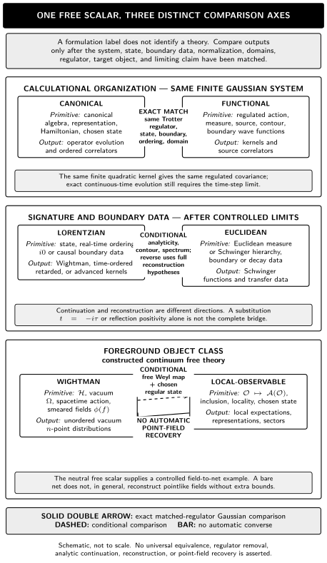
For one free scalar, canonical–functional agreement is exact only for the matched finite Trotter-regulated Gaussian system, while Lorentzian–Euclidean and Wightman–local-observable comparisons carry distinct hypotheses. Solid, dashed, and barred routes mark an exact matched-regulator comparison, a conditional comparison, and no automatic converse; the map is schematic and not to scale.

Read without the graphic: canonical and functional descriptions agree at finite regulator only when the Trotter kernel, state, boundary data, ordering, normalization, and domains match. Lorentzian continuation and Euclidean reconstruction are different conditional directions, and the neutral free scalar’s field-to-Weyl-net construction does not make point-field recovery from an abstract net automatic.

An arrow between rows is therefore conditional. A time-sliced functional integral can reproduce a canonical kernel when both use the same discretization and boundary states. Euclidean functions can determine Lorentzian data when the required analyticity, positivity, and reconstruction hypotheses hold. For the neutral free scalar, bounded Weyl generators associated with real smeared fields generate local observable algebras. More generally, charged or gauge-covariant fields can instead generate a field algebra, and obtaining the physical observable subalgebra requires separate locality, domain or strong-commutativity, and gauge-invariance hypotheses. None of these statements licenses a universal equivalence of all formulations.

A controlled free-scalar comparison

Take a massive real scalar in a finite spatial box and retain finitely many real normal modes. Before the continuum limit, the system is a finite collection of oscillators,

$$S_N = \frac12\int\mathrm dt \sum_{a=1}^{N} \left( \dot q_a^{\,2}-\omega_a^2q_a^2 \right).$$

Every retained mode has $\omega_a>0$. The canonical description adds

$$[q_a,p_b]=i\delta_{ab}.$$ $$H_N = \frac12\sum_{a=1}^{N} \left( p_a^2+\omega_a^2q_a^2 \right),$$

and chooses the normalized ground state $|0\rangle$. These additions are not decorative: the commutator fixes normalization, the Hamiltonian fixes time evolution, and the state fixes the expectation value. The construction of relativistic one- and many-particle states and the local free scalar from these oscillator data is developed in Coleman 2019, §§ 1.2–3.4, pp. 6–45.

For one mode, write

$$q(t) = \frac{1}{\sqrt{2\omega}} \left( ae^{-i\omega t} +a^\dagger e^{+i\omega t} \right).$$

The vacuum satisfies $a|0\rangle=0$. The positive-frequency Wightman function is

$$W(t) \equiv \langle0|q(t)q(0)|0\rangle = \frac{e^{-i\omega t}}{2\omega}.$$

Time ordering produces a different boundary value,

$$G_F(t) \equiv \langle0|Tq(t)q(0)|0\rangle = \frac{e^{-i\omega|t|}}{2\omega},$$

with the momentum representation

$$\begin{aligned} G_F(t) &= \int\frac{\mathrm dp^0}{2\pi}\, e^{-ip^0t}\,\widetilde G_F(p^0),\\ \widetilde G_F(p^0) &= \frac{i}{(p^0)^2-\omega^2+i0}. \end{aligned}$$

After the vacuum analytic continuation appropriate to this oscillator, the Euclidean covariance is

$$G_E(\tau) = \frac{e^{-\omega|\tau|}}{2\omega},$$

or equivalently

$$\begin{aligned} G_E(\tau) &= \int\frac{\mathrm dp_E}{2\pi}\, e^{ip_E\tau}\,\widetilde G_E(p_E),\\ \widetilde G_E(p_E) &= \frac{1}{p_E^2+\omega^2}. \end{aligned}$$

The inverse-kernel checks expose the different signatures:

$$\begin{aligned} (\partial_t^2+\omega^2)G_F(t)&=-i\delta(t),\\ (-\partial_\tau^2+\omega^2)G_E(\tau)&=\delta(\tau). \end{aligned}$$

The formulas agree on oscillator frequency and normalization, but each still remembers its state, ordering, contour, and signature. $W$ is not time ordered; $G_F$ contains the $i0$ boundary prescription; $G_E$ is selected by Euclidean decay. Deriving a functional integral by time slicing also introduces a precise Trotter kernel. At finite time step it matches the correspondingly discretized canonical kernel; equality with exact continuous-time canonical evolution requires the time-step limit. The time-sliced and Gaussian constructions are derived in Schwartz 2014, §§ 14.2–14.3, pp. 254–264.

What the comparison proves

At finite mode number, exact checks include:

• the same discrete oscillator frequencies $\omega_a$;
• the same canonical normalization and equal-time brackets;
• inversion of the corresponding regulated Lorentzian or Euclidean quadratic kernel;
• agreement between source derivatives and the chosen Gaussian covariance; and
• agreement of a time-sliced functional kernel with the same Trotterized canonical kernel and boundary data.

For this free Gaussian system, all higher correlators in the chosen Gaussian state are fixed by the two-point function through Wick factorization. Even here, matching a two-point expression only after silently changing its ordering or boundary value is not a valid comparison.

The finite system does not by itself establish a continuum relativistic field theory. A finite spatial mode cutoff replaces the Dirac delta by a truncated kernel, breaks exact boost invariance, and need not preserve exact continuum microcausality. Infinite-volume, ultraviolet-cutoff, and any zero-mass limits are separate. Only after the relevant distributional limits are controlled may one claim the continuum free field, its Wightman distributions, or causal support of its Pauli–Jordan commutator. This separation between a defined regulated model and a claimed limit is part of the theory’s meaning, not an afterthought.

The Wightman and local-observable endpoints

Suppose now that the massive neutral free scalar on Minkowski spacetime has been constructed after the relevant limits. Its Wightman description uses the vacuum, the unitary Poincaré action, and smeared operator-valued distributions. For test functions $f_i$,

$$W_n(f_1,\ldots,f_n) = \langle\Omega| \phi(f_1)\cdots\phi(f_n) |\Omega\rangle.$$

The positive-frequency two-point distribution fixes the higher $W_n$ in this quasifree vacuum by Wick factorization. This is the continuum endpoint of the unordered function $W(t)$ above, not an assertion that a finite spatial cutoff already obeys the Wightman axioms.

The same neutral scalar has a bounded local-algebra description. Let $P=\Box+m^2$, take real compactly supported test functions modulo additions of $Ph$, and let $\Delta(f,g)$ be the causal symplectic form. The abstract Weyl generators obey

$$\begin{aligned} \mathsf W([f])\mathsf W([g]) &= e^{-i\Delta(f,g)/2}\, \mathsf W([f+g]),\\ \mathsf W([f])^* &= \mathsf W([-f]). \end{aligned}$$

For a causally suitable open region $\mathcal O$, define

$$\mathcal A(\mathcal O) = C^*\!\left( \mathsf W([f]): \operatorname{supp}f\subset\mathcal O \right).$$

If the supports of $f$ and $g$ are spacelike separated, $\Delta(f,g)=0$, so the corresponding local algebras commute. In a regular vacuum representation, the one-parameter Weyl groups recover the represented smeared field generators; the identity $\mathsf W([f])=e^{i\phi(f)}$ is heuristic until that representation and its domains have been chosen. Thus the Wightman and local-observable descriptions share the same free equation, causal propagator, and vacuum state while foregrounding different objects. The free scalar field algebra, Weyl relations, local subalgebras, and quasifree states are constructed in Fewster and Rejzner 2020, §§ 4.2–4.3, pp. 15–23.

Consistency tests and failure diagnostics

The appropriate tests depend on the formulation, but the questions below catch many category errors.

Diagnostic question	Evidence that would answer it	Warning sign
Was the state held fixed?	The same vacuum, density operator, or boundary wave functions appear on both sides	“Vacuum” is assumed from notation, or an in–out object is compared with an in–in expectation
Are the outputs the same kind of object?	Ordering, support, contour, and source convention are declared	A Wightman, Feynman, retarded, and Euclidean kernel are called the same propagator
What is the strength of equality?	Exact finite identity, perturbative equality through a stated order, asymptotic statement, or theorem with hypotheses	A formal change of variables is described as complete framework equivalence
What does the regulator preserve?	Symmetry, positivity, locality, and Ward-identity checks are performed at finite regulator or after a controlled limit	Continuum covariance or microcausality is attributed to a noncovariant cutoff
Is the inserted quantity observable?	Adjointness, domains, gauge invariance, localization, and state-sector meaning are specified as relevant	Every field coordinate or gauge-fixed variable is called measurable
Has the desired limit been established?	Convergence, regulator independence of the declared observable, and renormalization conditions are exhibited	A long finite series or large lattice is treated as a proof of existence

Positivity deserves special care. In an operator formulation it can mean positivity of the state, $\omega(A^*A)\geq0$, and positive Hilbert-space norm. In Euclidean reconstruction it appears through a reflection-positivity condition. A gauge-fixed formulation requires a separate construction of its physical state space; no positivity conclusion is imported here from an auxiliary space. These are related requirements, not interchangeable slogans.

Common pitfalls

“The Lagrangian is the theory.” A Lagrangian is often excellent shorthand, but a definite prediction still requires state, boundary, prescription, regulator, renormalization, and observable data.

“Canonical and path-integral quantization are automatically equivalent.” Their agreement must be demonstrated for matched regulators, orderings, domains, contours, and boundary states. The finite oscillator comparison supplies one controlled case, not a universal theorem.

“Wick rotation is just $t=-i\tau$.” Analytic domains, singularities, contours, state selection, and positivity determine whether a continuation exists and what it reconstructs.

“A matching two-point function proves the theories are identical.” It can be decisive inside a declared free Gaussian class, where higher moments are fixed, but it does not by itself identify the full observable algebra, allowed states, global sectors, or interactions.

“A cutoff calculation is already the continuum theory.” It is a result about the regulated model unless regulator removal or a bounded effective-theory interpretation has been established.

Typed continuation

• Continue to Why Local Relativistic Quantum Theory Uses Fields for the physical motivation behind fields, particle-number-changing operators, and locality.
• Build the canonical free model in Canonical Quantization and the Free Scalar.
• Build its regulated functional description in Functional Integrals and Free Gaussian Fields.
• Separate Lorentzian, Euclidean, and in–in targets in Lorentzian, Euclidean, and In-In Formulations.
• Compare physical frameworks, with their hypotheses exposed, in Wightman, Euclidean, Local-Algebraic, Constructive, and Perturbative Frameworks.
• For theorem-level object classes and comparison maps, use QFT Frameworks, Object Classes, and Typed Maps.
• For the exact Euclidean reconstruction arrows and their nonconverses, use OS–Wightman Comparison Directions and Failure Modes.
• Diagnose interacting regulator removal through Regulators, Cutoffs, and Continuum Limits; that page routes the resulting construction to Renormalization and Effective Field Theory, Lattice and Hamiltonian QFT, or Mathematical QFT according to the required evidence.

Check your understanding

Prompt	A satisfactory answer includes	Repair
Given only $S[\phi]$, name four independent choices needed for a definite two-point function.	A state or boundary condition, ordering or contour, regulator/measure, and the field or observable insertion; renormalization and global data may also matter	Re-read Why an action is candidate data
Explain why one matched regulated two-point function does not prove universal equivalence.	The match is typed by state, ordering, regulator, observable class, and limit; non-Gaussian higher functions and global sectors can contain additional information	Re-read Formulation labels lie on different axes
Separate the free finite-mode checks from continuum claims.	Frequencies, brackets, Gaussian inversion, and matched Trotter kernels are finite checks; exact Poincaré covariance, continuum delta functions, and microcausality require controlled limits	Re-read What the comparison proves
A paper claims Euclidean data reconstruct a Lorentzian QFT. Where should the full theorem be checked?	The OS–Wightman comparison page, with reflection positivity, regularity, covariance, and reconstruction hypotheses stated	Follow the exact theorem-level treatment under Typed continuation

References

• Coleman, Sidney. Lectures of Sidney Coleman on Quantum Field Theory. Edited by Bryan Gin-ge Chen, David Derbes, David Griffiths, Brian Hill, Richard Sohn, and Yuan-Sen Ting. Singapore: World Scientific, 2019. DOI.
• Fewster, Christopher J., and Kasia Rejzner. “Algebraic Quantum Field Theory—an Introduction.” In Progress and Visions in Quantum Theory in View of Gravity, 1–61. Cham: Birkhäuser, 2020. DOI. Open PDF, arXiv:1904.04051v2.
• Hollands, Stefan, and Robert M. Wald. “Quantum Fields in Curved Spacetime.” Physics Reports 574 (2015): 1–35. DOI. Open PDF, arXiv:1401.2026v2.
• Schwartz, Matthew D. Quantum Field Theory and the Standard Model. Cambridge: Cambridge University Press, 2014. DOI.
• Weinberg, Steven. The Quantum Theory of Fields. Volume I: Foundations. Cambridge: Cambridge University Press, 1995. DOI.