The Spin–Statistics Connection

Spin does not determine statistics by itself. In a standard 3+1-dimensional, point-local Wightman setting, the connection follows from a conjunction of physical positivity, Poincaré covariance, a vacuum and forward spectrum, controlled field domains, nontriviality, and spacelike locality. For a field of definite spin parity, those assumptions force integer-spin fields to use the bosonic commutator sign and half-odd-integer-spin fields to use the fermionic anticommutator sign. This page maps one representative sufficient theorem package and tests it on free scalar and Dirac fields; it does not replace the rigorous theorem variants or their domain proofs.

Required background. Microcausality and Relativistic Compatibility supplies the smeared/common-domain meaning of a candidate locality bracket and the field–observable distinction. Hilbert Positivity and Unitary Evolution distinguishes the positive physical Hilbert space from an indefinite gauge-fixed auxiliary space. Canonical Quantization of the Free Dirac Field supplies the mode CAR, the vacuum-relative Hamiltonian, and the spacelike free-field check used below.

Spin and statistics enter through different structures

Spin is a transformation property. Let a finite-component field multiplet $F_a$ transform in a finite-dimensional Lorentz representation $(A,B)$ under the universal cover of the proper orthochronous Lorentz group. The central $2\pi$ rotation acts with parity

$$\chi_F=(-1)^{2(A+B)}=(-1)^{2s}.$$

Although the rotation decomposition can contain several spins, all have the same integer or half-integer parity. This finite-dimensional transformation on field components is not the unitary Poincaré representation on physical states. A reducible multiplet must first be decomposed into components with definite $2\pi$-rotation parity.

Statistics enters through a different relation. For a homogeneous field and its adjoint, define the candidate spacelike exchange bracket on a common invariant domain $\mathcal D$ by

$$[F_a(f),F_b^\dagger(g)]_\varepsilon := F_a(f)F_b^\dagger(g) -\varepsilon F_b^\dagger(g)F_a(f),$$

where $\varepsilon=+1$ means a commutator and $\varepsilon=-1$ means an anticommutator. The locality hypothesis is that this bracket vanishes when $\operatorname{supp}f$ and $\operatorname{supp}g$ are spacelike separated. For charged multiplets, mixed components and adjoints must be stated in the chosen theorem; the compact notation above is only the definite-parity core. It does not preassign $\varepsilon$ from the spin.

The spin–locality conclusion is

$$\boxed{\varepsilon=\chi_F=(-1)^{2s}}.$$

Thus the declared spacelike $F$–$F^\dagger$ bracket is a commutator for integer spin and an anticommutator for half-odd-integer spin in this setting. In the usual free Fock realizations this local field grading agrees with symmetric or antisymmetric multiparticle states. That particle statement is not identical to the field theorem in every framework: charged sectors, braid statistics, and generalized statistics require their own formulation. Greenberg 1998, printed pp. 1–6 (open manuscript PDF) separates spin–locality, particle statistics, and CPT rather than treating them as one assertion.

Historically, Pauli established a free relativistic field/particle result using positive energy and spacelike commutativity; it was not the later Wightman-domain theorem Pauli 1940, pp. 716–722. Lüders and Zumino subsequently treated the interacting single-field problem for spin zero and one-half under axiomatic hypotheses Lüders and Zumino 1958, abstract. The open Greenberg and Schroer sources below support the wrong-bracket triviality step; the short historical paper is not used as the sole source for the broader theorem map.

A representative four-dimensional theorem package

One useful sufficient package begins with all of the following, not with any single row in isolation:

1. Dimension and topology. Spacetime is 3+1-dimensional Minkowski space, and the theorem uses the ordinary two-sign point-local grading; this is not a 2+1-dimensional braided-sector theorem.
2. Physical positivity. Fields act in a Hilbert space with a positive-definite inner product; an indefinite auxiliary form is not a substitute.
3. Covariance and spin parity. A strongly continuous unitary representation of the Poincaré cover acts on states, while the field has a declared finite-dimensional covariant transformation law and definite $2\pi$-rotation parity.
4. Vacuum and spectrum. There is an invariant cyclic vacuum, conventionally unique up to phase in this representative version, and the joint translation spectrum lies in the closed forward cone.
5. Fields and domains. The field is a nonzero operator-valued tempered distribution on a common invariant dense domain; the field, adjoint, and complete field system obey the theorem’s specified relative-locality relations on that domain.
6. Candidate spacelike locality. The bracket with one declared sign $\varepsilon$ vanishes after smearing with spacelike-separated supports.

Greenberg 1998, arXiv v2, printed pp. 2–4 (PDF) states the positive-metric, domain, covariance, vacuum-spectrum, and locality ingredients and distinguishes the wrong-bracket triviality statement from particle statistics. The list above is a deliberately non-minimal synthesis of that standard Wightman-style setting, not a claim that every theorem variant uses an identical axiom list.

For example, if

$$W_{2,ab}(x-y) := \langle\Omega|F_a(x)F_b^\dagger(y)|\Omega\rangle,$$

then the forward-spectrum condition gives, with the site’s Fourier phase,

$$\operatorname{supp}\widetilde W_2 \subseteq\overline V_+.$$

This support statement is one input to analytic continuation; it does not by itself choose the exchange sign. Likewise, spacelike locality by itself only tests a proposed sign. The theorem connects the two after covariance, positivity, and the field assumptions are added.

The diagram makes that logical conjunction visible. Follow the solid inputs into the proof band, then inspect the separate dashed qualification cards: they mark a change of theorem, not a contradiction.

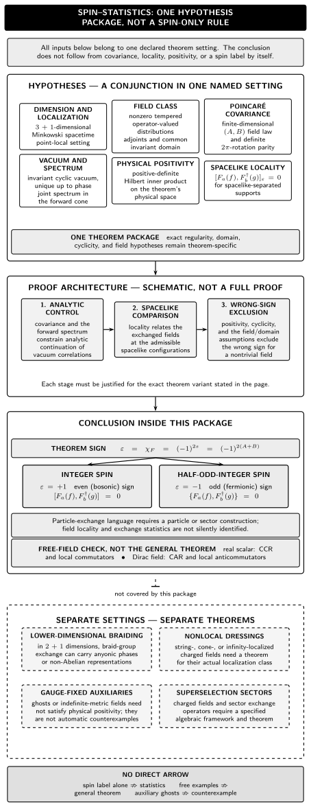
Within the declared 3+1-dimensional point-local package, covariance and the spectrum condition supply analytic control, locality compares spacelike field orderings, and physical positivity together with cyclicity and the field/domain assumptions exclude the wrong sign for a nontrivial field. The resulting $\varepsilon=(-1)^{2s}=(-1)^{2(A+B)}$ gives $\varepsilon=+1$ and a vanishing spacelike commutator for integer spin, while $\varepsilon=-1$ gives a vanishing spacelike anticommutator for half-odd-integer spin. Low-dimensional braid statistics, gauge-fixed auxiliary fields, nonlocal dressings, and superselection formulations require different hypotheses and theorems. The map is schematic and not a proof or universal classification.

Semantic account of every input, conclusion, and qualification in the spin–statistics logic map.

Element	Role in the displayed package	Licensed conclusion	What does not follow
3+1 dimensions and exchange topology	Fixes the ordinary two-sign point-local grading; a particle-exchange interpretation needs a sector or particle construction.	The conclusion may be expressed by a sign, plus or minus one.	The same dichotomy in two spatial dimensions.
Field class and domains	Supplies nonzero covariant distributions, adjoints, a common domain, and cyclicity and relative-locality control.	The analytic vacuum statement can be promoted to a field statement in the specified theorem.	A theorem for arbitrary nonlocal, string-localized, or dressed fields.
Poincaré covariance and spin parity	Provides the proper-orthochronous cover action and the sign of a full rotation.	The analytic exchange comparison carries an integer- or half-integer-spin parity.	Spin representation alone fixes statistics.
Invariant vacuum and forward spectrum	Give spectral support and analytic control of vacuum correlation functions.	Boundary values can be compared in the theorem’s analytic domain.	A mass gap, asymptotic particles, or scattering completeness.
Positive physical Hilbert space	Turns the relevant vacuum expression into a nonnegative norm and excludes negative-norm escape routes.	The wrong sign forces every relevant field-created vacuum vector to vanish in the complete theorem package.	The same conclusion in an indefinite gauge-fixed auxiliary space.
Candidate spacelike locality sign	Compares exchanged fields at admissible spacelike configurations.	Together with every other input, the sign must match the spin parity for a nontrivial field.	Microcausality alone proves spin–statistics.
Scoped conclusion	All six inputs meet in one Wightman-style theorem.	The declared spacelike field–adjoint bracket is a commutator for integer spin and an anticommutator for half-odd-integer spin.	A universal classification of every notion of particle statistics.
Free-field check	The real scalar uses a spacelike commutator and the Dirac field a spacelike anticommutator.	The two free Fock constructions realize the theorem’s two signs.	A proof of the general interacting theorem.
Low-dimensional braid statistics	Changes the topology and the exchange group.	A separate spin–braid relation may replace the plus-or-minus sign.	A counterexample to the four-dimensional theorem.
Gauge auxiliaries and ghosts	May violate physical positivity before the constraint, quotient, or cohomology is taken.	The theorem is applied only after physical states and observables are identified.	A scalar Grassmann ghost refutes spin–statistics.
Nonlocal dressings	May fail compact spacelike locality even when physically necessary.	A theorem adapted to the actual localization class is required.	The point-local theorem applies unchanged.
Superselection and generalized statistics	Encode exchange in sectors or categories rather than one point-field bracket.	Separate algebraic spin–statistics results may apply.	A preferred point field or ordinary two-sign grading follows automatically.
No-direct-arrow strip	Blocks spin label alone, free examples alone, and auxiliary ghosts from being treated as a general proof or counterexample.	No additional conclusion; the full declared package remains necessary.	Any one of those three shortcuts establishes or refutes the theorem.

The proof architecture uses every hypothesis

A standard Wightman-style proof pattern is not a mode-counting argument. Its main steps are:

1. The spectrum condition turns vacuum correlation distributions into boundary values of holomorphic functions in tube domains.
2. Covariance under the complexified Lorentz group compares analytically related spacelike configurations. A full rotation contributes the field’s $2\pi$ sign $(-1)^{2s}$.
3. Spacelike locality compares the reversed field order with the independently declared sign $\varepsilon$.
4. Boundary-value uniqueness carries that comparison back to the physical distributions.
5. Positivity converts the wrong-sign relation into a vanishing norm. In the complete relatively local field system, cyclicity and the relevant Reeh–Schlieder consequence then promote $F_a(f)\Omega=0$ for all $f$ to triviality of the field.

In particular, the intermediate conclusion has the form

$$\varepsilon\ne(-1)^{2s} \quad\Longrightarrow\quad F_a(f)\Omega=0 \qquad\text{for every test function }f.$$

The last step is deliberately stated in two parts: positivity alone does not make an operator vanish. The common domain, analytic continuation, nontriviality, and cyclic field system do real work. Nor is graded locality a circular shortcut. One first proposes a locality sign, and the theorem asks whether that sign is compatible with the independently specified spin parity and physical structure. Schroer 1998, § 5.2, p. 191 (open lecture-note PDF) gives this tube-analytic, complex-Lorentz, positivity, and Reeh–Schlieder skeleton for the neutral two-point illustration; general multiplets require the full theorem’s component and relative-locality hypotheses.

First application: scalar commutators and Dirac anticommutators

The free fields give a transparent check of the conclusion, not its general proof. Let

$$\mathrm d\Pi_{\mathbf p} := \frac{\mathrm d^3\mathbf p}{(2\pi)^3 2E_{\mathbf p}}, \qquad E_{\mathbf p}=\sqrt{|\mathbf p|^2+m^2},$$

and use the Pauli–Jordan convention from the microcausality prerequisite,

$$i\Delta_m(z) = \int\mathrm d\Pi_{\mathbf p} \left(e^{-ip\cdot z}-e^{ip\cdot z}\right).$$

The scalar selects the commutator

For the free real scalar,

$$[\phi(x),\phi(y)] =i\Delta_m(x-y)\mathbf1.$$

Because $\operatorname{supp}\Delta_m\subseteq\{z:z^2\ge0\}$, this commutator vanishes at spacelike separation. The opposite candidate bracket does not. Its vacuum matrix element is

$$\begin{aligned} \langle\Omega|\{\phi(x),\phi(y)\}|\Omega\rangle &=W_0(z)+W_0(-z)\equiv\Delta_m^{(1)}(z),\\ \Delta_m^{(1)}(0,\mathbf r) &=\frac{m}{2\pi^2r}K_1(mr)>0 \qquad(m>0,\ r=|\mathbf r|>0). \end{aligned}$$

Thus the integer-spin scalar is local with the commutator, not the anticommutator. A deliberately nonlocal positive-energy scalar model with a Fermi assignment evades this conclusion by losing local observable/energy density; it is outside the theorem rather than a counterexample Greenberg 1998, arXiv v2, printed pp. 5–6 (PDF).

The Dirac field selects the anticommutator

Write

$$D(z) := \int\mathrm d\Pi_{\mathbf p} \left(e^{-ip\cdot z}-e^{ip\cdot z}\right) =i\Delta_m(z).$$

The free Dirac mode CAR and spin sums give

$$\{\psi_\alpha(x),\bar\psi_\beta(y)\} = \left[ \left(i\gamma^\mu\partial_{x^\mu}+m\right)D(x-y) \right]_{\alpha\beta}.$$

Differentiation does not enlarge distributional support, so the anticommutator vanishes at spacelike separation. At equal time it reproduces

$$\{\psi_\alpha(t,\mathbf x), \psi_\beta^\dagger(t,\mathbf y)\} = \delta_{\alpha\beta}\delta^{(3)}(\mathbf x-\mathbf y).$$

Free even bilinears such as $j^\mu=:\!\bar\psi\gamma^\mu\psi\!:$ have vanishing commutators after smearing with spacelike-separated supports: exchanging two odd factors twice gives the ordinary observable sign. The free scalar and spinor causal-bracket calculations appear together in Schwartz 2014, § 12.6, printed pp. 219–222.

The negative-frequency Dirac oscillator supplies a second, independent test. Before reordering, its contribution is

$$H_-=-E\,d d^\dagger.$$

With CAR, $dd^\dagger=1-d^\dagger d$, so the vacuum-relative excitation has positive energy and the mode has only occupations zero and one. If instead $[d,d^\dagger]=+1$, then

$$H_-=-E(d^\dagger d+1),$$

which is unbounded below as the bosonic occupation grows. Reversing the commutator sign repairs the excitation gap only by producing

$$\|d^\dagger\Omega\|^2 = \langle\Omega|dd^\dagger|\Omega\rangle =-1.$$

The free commutator choice therefore cannot preserve both positive norm and positive excitation energy. This regulated one-mode diagnostic is useful but is not the relativistic theorem: it does not supply the analytic, locality-domain, and cyclicity steps above. Schwartz 2014, § 12.5.2, printed pp. 217–218 gives the same wrong-statistics energy test.

Qualifications are changes of theorem, not paradoxes

Two spatial dimensions. Localized sectors may carry braid-group statistics, although ordinary Bose and Fermi sectors remain possible. With Mund’s exchange-orientation convention, his massive charged-sector theorem—with a positive mass separated from the rest of its sector’s mass spectrum by a gap, only finitely many particle types in that sector at that mass, and common spin—gives $\omega=e^{2\pi i s}$ for the braid statistics phase. Non-Abelian braid representations require still more data. These are anyonic or braided theorem variants, not violations of the four-dimensional result. Mund 2009, § 1, printed pp. 1–2 (PDF) states that scoped relation, while Fewster and Rejzner 2019, arXiv v2, §§ 8.2–8.3, printed pp. 37–40 (PDF) explain how spacetime dimension changes the sector-statistics structure.

Gauge-fixed auxiliary fields and ghosts. Faddeev–Popov ghosts are Lorentz scalars but Grassmann odd. They do not act as point-local scalar particles in a positive physical Hilbert space; they belong to an auxiliary indefinite or cohomological construction. The physical theorem is applied only after the physical state space and observable algebra are identified. Likewise, Berezin variables in a functional integral encode an algebraic sign but do not, by themselves, prove a physical spin–statistics connection. Greenberg 1998, arXiv v2, printed pp. 3–4 (PDF) makes the positive-metric failure in the ghost example explicit.

Nonlocal fields and dressings. String-, cone-, or infinity-localized fields do not satisfy the compact point-local hypothesis merely by being physically motivated. A theorem adapted to the actual localization class is required; local gauge-invariant observables may still satisfy ordinary microcausality. The explicit wrong-statistics scalar escape by nonlocal energy density is analyzed in Greenberg 1998, arXiv v2, printed pp. 5–6 (PDF).

Parastatistics and superselection sectors. A sector formulation can place statistics in localized endomorphisms and exchange operators rather than in a single point field. Recovering ordinary Bose/Fermi fields, internal gauge degrees of freedom, or para-equivalences takes additional hypotheses. The two-sign field formula on this page is not that theorem. Fewster and Rejzner 2019, arXiv v2, §§ 8.2–8.3, printed pp. 37–40 (PDF) give the bounded sector and generalized-statistics orientation.

No mass gap or asymptotic completeness was used in the representative spin–locality package. Adding particle scattering can require both. Conversely, a nonrelativistic many-body model, a lattice model without exact Lorentz symmetry, or a topological effective theory can have well-defined exchange rules without satisfying this page’s assumptions.

Check your understanding

Why does microcausality not already prove the theorem?

Microcausality only says that a chosen commutator or graded bracket vanishes at spacelike separation. The theorem must still relate that independently chosen sign to the $2\pi$ rotation parity using covariance, the forward spectrum, analytic continuation, positivity, and field-domain assumptions.

Why is a scalar Grassmann ghost not a counterexample?

The usual physical theorem assumes a positive-definite physical Hilbert space and a physical point-local field. A gauge-fixed ghost is auxiliary and violates that hypothesis; its grading helps encode gauge cancellations rather than describing a scalar physical particle with Fermi statistics.

Which free-field calculation checks the two locality signs?

The scalar commutator is $i\Delta_m$ and vanishes spacelike, while the scalar anticommutator has a nonzero spacelike vacuum matrix element. For the Dirac field, the anticommutator is the Dirac operator applied to $D=i\Delta_m$, so it has causal support. The antiparticle oscillator then shows why commutators cannot retain both positive norm and a lower-bounded vacuum-relative energy.

Where to continue

• Strengthen the field-locality input: Microcausality and Relativistic Compatibility distinguishes graded fields from physical even observables and states the common-domain caveat.
• Recheck the explicit fermion construction: Canonical Quantization of the Free Dirac Field derives the CAR, Hamiltonian, charge, and spacetime anticommutator in full.
• Enter the rigorous theorem variants: Spin–Statistics Theorems and Failure Modes develops the precise domain, low-dimensional, and superselection formulations that are only mapped here.

References

• Fewster, Christopher J., and Kasia Rejzner. “Algebraic Quantum Field Theory—an Introduction.” arXiv:1904.04051v2, 2019; published in Progress and Visions in Quantum Theory in View of Gravity, edited by Felix Finster, Domenico Giulini, Johannes Kleiner, and Jürgen Tolksdorf, 1–61. Birkhäuser, 2020. DOI. Open manuscript PDF, v2.
• Greenberg, O. W. “Spin-Statistics, Spin-Locality, and TCP: Three Distinct Theorems.” Physics Letters B 416 (1998): 144–149. DOI. Open manuscript PDF, v2.
• Lüders, Gerhart, and Bruno Zumino. “Connection between Spin and Statistics.” Physical Review 110 (1958): 1450–1453. DOI.
• Mund, Jens. “The Spin-Statistics Theorem for Anyons and Plektons in d = 2+1.” Communications in Mathematical Physics 286 (2009): 1159–1180. DOI. Open manuscript PDF, v2.
• Pauli, Wolfgang. “The Connection Between Spin and Statistics.” Physical Review 58 (1940): 716–722. DOI.
• Schroer, Bert. Localization and Nonperturbative Local Quantum Physics. Lecture notes, arXiv:hep-th/9805093, 1998. DOI. Open manuscript PDF.
• Schwartz, Matthew D. Quantum Field Theory and the Standard Model. Cambridge University Press, 2014. DOI.