The Klein–Gordon Field and Its Modes

In flat spacetime, every sufficiently regular solution of the free massive real-scalar equation is a superposition of the two branches of the mass shell. Reality pairs the positive- and negative-frequency coefficients, while a conserved symplectic form fixes their relative normalization. Choosing the future-directed time-translation branch as “positive frequency” supplies additional structure that later quantization will use; it is not yet an operator algebra, vacuum, or particle interpretation.

This page develops that classical construction for $m>0$, first with continuum plane waves and then in a periodic spatial box. It stops before canonical commutators and defers the massless zero mode and general curved-spacetime mode ambiguity.

Required background. The Action Principle and Field Equations supplies the variation of the scalar action, including the surface term whose vanishing is assumed below.

Helpful background. Fourier Series, Fourier Transforms, and Plancherel Theory supplies continuum and periodic normalization; Linear ODEs, Evolution Operators, and Wronskians explains conserved mode pairings; Sturm–Liouville Problems and Eigenfunction Expansions supplies boundary-adapted bases; Symbols, Characteristics, and PDE Type distinguishes dispersion from characteristics; and Normal Forms, Spectra, and Projectors supplies spectral-subspace language.

Plane waves on the Klein–Gordon mass shell

The reference model has one real scalar field on $d$-dimensional Minkowski spacetime, a chosen future time orientation, and mass $m>0$. Its defining action and field equation are

$$\begin{aligned} S_0[\phi] &= \frac12\int \mathrm d^d x\, \left( \partial_\mu\phi\,\partial^\mu\phi-m^2\phi^2 \right), \\ (\Box+m^2)\phi &=0. \end{aligned}$$

The variational derivation is given on the required-background page. Here the relevant boundary hypothesis is that the variation has compact support, the fields decay sufficiently fast, or the chosen boundary conditions cancel the surface term. The model is invariant under Poincaré transformations and under $\phi\mapsto-\phi$. Its classical data are $\phi$ and $\partial_t\phi$ on a Cauchy slice; the periodic-box version below replaces decay at spatial infinity by periodicity.

For a plane wave $u_p(x)=e^{-ip\cdot x}$,

$$(\Box+m^2)u_p = (-p^2+m^2)u_p.$$

Thus a nonzero plane-wave solution obeys

$$p^2=m^2, \qquad p^0=\pm E_{\mathbf p}, \qquad E_{\mathbf p}=\sqrt{\mathbf p^2+m^2}.$$

The two sheets are the positive- and negative-frequency branches relative to the chosen coordinate $t$. This mass shell is not the characteristic cone of the differential equation: the principal symbol ignores the lower-order mass term, so the characteristics remain null even when $m>0$. The distinction matters when one passes from oscillatory solutions to propagation of singularities.

Plane waves are generalized modes rather than finite-energy configurations. Ordinary classical data are represented by wave packets with suitable falloff, or by the normalizable finite-volume modes constructed below. The massive action and equation are derived in Schwartz 2014, § 3.2, pp. 31–32; Srednicki 2006, § 3, pp. 37–40 additionally develops the massive dispersion relation and real-field mode expansion after translation to the site convention. The plane-wave oscillator reduction begins in Schwartz 2014, § 2.2, pp. 17–19.

Real solutions require both frequency branches

Complex solutions are a convenient intermediate language even though the physical classical field is real. Put $p^0=E_{\mathbf p}$ and define the invariant on-shell measure

$$\int_{\mathbf p} \equiv \int \frac{\mathrm d^{d-1}\mathbf p} {(2\pi)^{d-1}2E_{\mathbf p}}.$$

A sufficiently regular real solution can then be written

$$\phi(x) = \int_{\mathbf p} \left[ c(\mathbf p)e^{-ip\cdot x} +c(\mathbf p)^*e^{ip\cdot x} \right].$$

Here $c(\mathbf p)$ is a classical complex-valued amplitude, and $^*$ means complex conjugation. The second term is forced by $\phi^*=\phi$; it is not an independent “negative-energy field.” In particular,

$$\phi=\phi_++\phi_-, \qquad \phi_-=\phi_+^*,$$

with $i\partial_t\phi_+=+E\phi_+$ mode by mode and $i\partial_t\phi_-=-E\phi_-$ mode by mode. The names positive and negative frequency therefore refer to eigenvalues of the selected time-translation generator on the complexified solution space.

For wave packets the classical energy provides a useful sign check:

$$\begin{aligned} H &= \frac12\int \mathrm d^{d-1}\mathbf x\, \left[ (\partial_t\phi)^2 +|\boldsymbol\nabla\phi|^2 +m^2\phi^2 \right] \\ &= \int_{\mathbf p} E_{\mathbf p}|c(\mathbf p)|^2 \geq 0. \end{aligned}$$

Both frequency branches participate in this real, positive-energy solution. The conjugacy relation, invariant measure, and recovery of the classical coefficients are displayed in Srednicki 2006, § 3, pp. 38–40; Srednicki uses the opposite metric signature, so the invariant check after translation is $p^2=m^2$ here.

Symplectic conservation and the Klein–Gordon form

Let $\phi_1$ and $\phi_2$ be real solutions. Their bilinear current

$$j^\mu(\phi_1,\phi_2) = \phi_1\partial^\mu\phi_2 -(\partial^\mu\phi_1)\phi_2$$

is conserved on shell because

$$\partial_\mu j^\mu = \phi_1\Box\phi_2-(\Box\phi_1)\phi_2 =0.$$

On a Cauchy surface $\Sigma$, this current defines the antisymmetric form

$$\Omega_\Sigma(\phi_1,\phi_2) = \int_\Sigma \mathrm d\Sigma_\mu\, j^\mu(\phi_1,\phi_2).$$

For a constant-time slice,

$$\Omega_t(\phi_1,\phi_2) = \int \mathrm d^{d-1}\mathbf x\, \left( \phi_1\partial_t\phi_2 -(\partial_t\phi_1)\phi_2 \right).$$

The divergence theorem makes $\Omega_\Sigma$ independent of the Cauchy surface only when the flux through the remaining boundary vanishes. Sufficient decay, compactly supported Cauchy data, or periodic cancellation provides that condition in the cases used here. A reflecting or open boundary with nonzero flux requires a separate boundary analysis; current conservation alone is not enough.

After complexifying the solution space, define the Hermitian Klein–Gordon form by

$$(f,g)_{\mathrm{KG}} = i\,\Omega_\Sigma(f^*,g) = i\int_\Sigma \mathrm d\Sigma_\mu \left[ f^*\partial^\mu g -(\partial^\mu f^*)g \right].$$

This form is nondegenerate under the stated Cauchy and boundary hypotheses, but it is not positive on the full complex solution space. Positive-frequency modes have positive norm; their complex conjugates have negative norm. Only its restriction to a compatible positive-frequency subspace is a positive inner product. The relation between the classical solution pairing, Cauchy data, and the later field algebra is stated in Hollands and Wald 2015, § 2.1, pp. 9–12, Open PDF.

The current $j^\mu(\phi_1,\phi_2)$ should also not be confused with a physical $U(1)$ Noether current. It is a bilinear pairing of two solutions. A single real scalar has no continuous phase symmetry; the charged complex field is treated later.

Continuum mode normalization

For $u_{\mathbf p}(x)=e^{-ip\cdot x}$ with $p^0=E_{\mathbf p}$, the constant-time form gives

$$\begin{aligned} (u_{\mathbf p},u_{\mathbf q})_{\mathrm{KG}} &= (E_{\mathbf p}+E_{\mathbf q}) e^{i(E_{\mathbf p}-E_{\mathbf q})t} \int \mathrm d^{d-1}\mathbf x\, e^{i(\mathbf q-\mathbf p)\cdot\mathbf x} \\ &= (2\pi)^{d-1}2E_{\mathbf p}\, \delta^{(d-1)}(\mathbf p-\mathbf q). \end{aligned}$$

The remaining pairings are

$$\begin{aligned} (u_{\mathbf p}^*,u_{\mathbf q}^*)_{\mathrm{KG}} &= -(2\pi)^{d-1}2E_{\mathbf p}\, \delta^{(d-1)}(\mathbf p-\mathbf q), \\ (u_{\mathbf p},u_{\mathbf q}^*)_{\mathrm{KG}} &=0. \end{aligned}$$

These equations explain the factor $2E_{\mathbf p}$ in the on-shell measure. Applying the pairing to the real solution recovers its coefficient directly,

$$(u_{\mathbf p},\phi)_{\mathrm{KG}} =c(\mathbf p),$$

and the positive-frequency part obeys

$$(\phi_+,\phi_+)_{\mathrm{KG}} = \int_{\mathbf p}|c(\mathbf p)|^2.$$

An equivalent convention puts $1/\sqrt{2E_{\mathbf p}}$ into each mode and integrates with $\mathrm d^{d-1}\mathbf p/(2\pi)^{d-1}$. The corresponding modes are delta-normalized without the factor $2E_{\mathbf p}$. Either package is valid; moving a factor between the measure and the modes without translating the coefficients breaks coefficient recovery and, later, the canonical commutator. The positive-energy mode normalization used in the quantum scalar construction is displayed in Weinberg 1995, § 5.2, p. 201.

Periodic-box modes

Now take space to be a $(d-1)$-torus with common period $L$ and volume $V=L^{d-1}$. Periodic boundary conditions give

$$\mathbf k_{\mathbf n} = \frac{2\pi}{L}\mathbf n, \qquad \omega_{\mathbf n} = \sqrt{\mathbf k_{\mathbf n}^2+m^2}, \qquad \mathbf n\in\mathbb Z^{d-1}.$$

The spatial Fourier expansion

$$\phi(t,\mathbf x) = \frac{1}{\sqrt V} \sum_{\mathbf n} q_{\mathbf n}(t)e^{i\mathbf k_{\mathbf n}\cdot\mathbf x}, \qquad q_{-\mathbf n}=q_{\mathbf n}^*,$$

turns the field equation into one oscillator equation per momentum,

$$\ddot q_{\mathbf n} +\omega_{\mathbf n}^2q_{\mathbf n} =0.$$

Define the Klein–Gordon-normalized positive-frequency modes

$$v_{\mathbf n}(t,\mathbf x) = \frac{ e^{-i\omega_{\mathbf n}t +i\mathbf k_{\mathbf n}\cdot\mathbf x} } {\sqrt{2\omega_{\mathbf n}V}}.$$

Direct integration over the box gives

$$\begin{aligned} (v_{\mathbf n},v_{\mathbf m})_{\mathrm{KG}} &=\delta_{\mathbf n\mathbf m}, \\ (v_{\mathbf n}^*,v_{\mathbf m}^*)_{\mathrm{KG}} &=-\delta_{\mathbf n\mathbf m}, \\ (v_{\mathbf n},v_{\mathbf m}^*)_{\mathrm{KG}} &=0. \end{aligned}$$

Consequently every smooth real solution in the box has the expansion

$$\phi(x) = \sum_{\mathbf n} \left[ z_{\mathbf n}v_{\mathbf n}(x) +z_{\mathbf n}^*v_{\mathbf n}(x)^* \right], \qquad z_{\mathbf n}=(v_{\mathbf n},\phi)_{\mathrm{KG}},$$

and its energy is $H=\sum_{\mathbf n}\omega_{\mathbf n}|z_{\mathbf n}|^2$ whenever the sum converges. This is the finite-volume normalization round trip: the mode coefficient, Klein–Gordon norm, and energy all use the same factor $1/\sqrt{2\omega_{\mathbf n}V}$.

The continuum and box conventions match under

$$\begin{aligned} \int \frac{\mathrm d^{d-1}\mathbf p}{(2\pi)^{d-1}} &\longrightarrow \frac1V\sum_{\mathbf n}, \\ (2\pi)^{d-1} \delta^{(d-1)}(\mathbf p-\mathbf q) &\longrightarrow V\delta_{\mathbf n\mathbf m}. \end{aligned}$$

Finite volume discretizes momentum but does not impose a finite mode cutoff: the set $\mathbb Z^{d-1}$ is still infinite. A cutoff is a separate regulator. The box also selects a frame and breaks continuous boost symmetry, so box calculations should not be advertised as exactly Lorentz invariant. For $m>0$, the spatial zero mode has frequency $m$; at $m=0$ it requires the separate analysis on the infrared page. A torus mode normalization with the same $1/\sqrt{2\omega V}$ structure appears in Hollands and Wald 2015, pp. 45–46, Open PDF.

The normalization map below separates what has been derived here from the quantum checks it must later pass. Inspect the solid upper route for the classical coefficient and energy round trip; the dashed lower route is a handoff to the canonical algebra and quantized-field pages, not a derivation of commutators from classical mechanics.

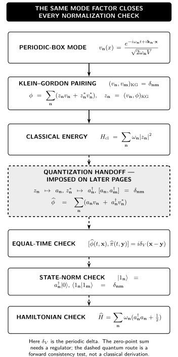
For the massive real scalar in a periodic box, $1/\sqrt{2\omega_{\mathbf n}V}$ makes the positive-frequency modes Klein–Gordon orthonormal, recovers $z_{\mathbf n}$ by pairing, and gives $H_{\mathrm{cl}}=\sum\omega_{\mathbf n}|z_{\mathbf n}|^2$. After quantization is separately imposed, the same normalization yields the periodic equal-time commutator, unit one-particle norms, and the oscillator Hamiltonian mode by mode. The lower dashed route is a forward consistency check; the infinite zero-point sum requires a regulator. The diagram is schematic and not to scale.

Normalization step	Exact statement	Status on this page
Box mode	$v_{\mathbf n}=e^{-i\omega_{\mathbf n}t+i\mathbf k_{\mathbf n}\cdot\mathbf x}/\sqrt{2\omega_{\mathbf n}V}$	Defined and checked classically
Klein–Gordon pairing	$(v_{\mathbf n},v_{\mathbf m})_{\mathrm{KG}}=\delta_{\mathbf n\mathbf m}$	Derived here
Coefficient and energy	$z_{\mathbf n}=(v_{\mathbf n},\phi)_{\mathrm{KG}}$ and $H_{\mathrm{cl}}=\sum\omega_{\mathbf n}	z_{\mathbf n}
Quantum input	$z_{\mathbf n}$ and $z_{\mathbf n}^*$ are replaced by $a_{\mathbf n}$ and $a_{\mathbf n}^\dagger$, with $[a_{\mathbf n},a_{\mathbf m}^\dagger]=\delta_{\mathbf n\mathbf m}$	A later quantization postulate, not a classical conclusion
Regression checks	$[\widehat\phi(t,\mathbf x),\widehat\pi(t,\mathbf y)]=i\delta_V(\mathbf x-\mathbf y)$, unit one-particle norm, and $\widehat H=\sum\omega_{\mathbf n}(a_{\mathbf n}^\dagger a_{\mathbf n}+1/2)$	Verified on later pages; $\delta_V$ is the periodic delta and the zero-point sum must be regulated

What the positive-frequency choice depends on

The real solution space and its symplectic form do not by themselves label half the complexified solutions as positive frequency. Such a label is a choice of a compatible complex structure. Equivalently, one selects a positive Lagrangian subspace $\mathcal S_+$ such that

$$\begin{aligned} \mathcal S_{\mathbb C} &= \mathcal S_+ \oplus \overline{\mathcal S_+}, \\ \Omega(\mathcal S_+,\mathcal S_+) &=0, \\ (f,f)_{\mathrm{KG}} &>0 \quad \text{for every }0\ne f\in\mathcal S_+. \end{aligned}$$

The isotropy condition makes the positive- and negative-frequency sectors Klein–Gordon orthogonal. In Minkowski spacetime, a future time orientation and the global time-translation generator select the standard $E_{\mathbf p}>0$ branch. That is the choice used throughout the rest of this free-scalar chapter.

The distinction becomes visible when no preferred time flow exists. A general time-dependent curved spacetime can retain a conserved symplectic form while admitting no distinguished positive-frequency split. The resulting mode and vacuum ambiguity is developed in Vacuum Ambiguity, Time Flow, and Observer Dependence. In flat spacetime the practical mode construction is given in Hollands and Wald 2015, pp. 16–17, Open PDF.

Common pitfalls

Treating the Klein–Gordon form as positive on every complex solution. Conjugate negative-frequency modes have negative norm. Positivity holds only after choosing and restricting to a compatible positive-frequency subspace.

Calling negative frequency negative energy. The present field is classical, and reality requires both frequency branches. Its Hamiltonian is nonnegative for $m^2\geq0$ under the stated boundary conditions; no antiparticle or negative-energy quantum state has been introduced.

Turning classical amplitudes into operators by typography. The coefficients $c(\mathbf p)$ and $z_{\mathbf n}$ are complex numbers, so their partners carry $^*$, not $^\dagger$. Operators and commutators begin on later pages.

Discarding boundary flux or conflating regulators. A locally conserved current yields a slice-independent pairing only when the external flux vanishes. Periodic volume, a finite mode cutoff, the infinite-volume limit, and the massless limit are four different choices or operations.

Check your understanding

Use each stated criterion and repair link to diagnose the corresponding derivation.

1. Retrieve the mass shell. Substitute $e^{-ip\cdot x}$ into the field equation. A satisfactory calculation obtains $p^2=m^2$ and both signs of $p^0$ without changing the inherited metric convention. Repair: return to Plane waves on the Klein–Gordon mass shell.

2. Distinguish the forms. Explain why $\Omega$ is real and antisymmetric on real solutions, while $(\cdot,\cdot)_{\mathrm{KG}}$ is Hermitian but indefinite on the complexification. A satisfactory answer identifies the positive-frequency restriction needed for a positive inner product. Repair: return to Symplectic conservation and the Klein–Gordon form.

3. Reconstruct the normalization. Starting with $u_{\mathbf p}=e^{-ip\cdot x}$, derive its Klein–Gordon pairing and recover $c(\mathbf p)=(u_{\mathbf p},\phi)_{\mathrm{KG}}$. A satisfactory result contains the same $(2\pi)^{d-1}2E_{\mathbf p}$ in the delta normalization that appears inversely in the on-shell measure. Repair: return to Continuum mode normalization.

4. Find the failure condition. Compare the pairing on two Cauchy slices when flux escapes through an external boundary. A satisfactory answer says that current conservation makes their difference equal to that boundary flux, so slice independence fails unless the flux vanishes. Repair: return to the conservation argument above or to Boundaries, Variations, and Well-Posed Actions.

5. Transfer to a box. Replace the continuum integral and delta distribution by their periodic counterparts and check $(v_{\mathbf n},v_{\mathbf m})_{\mathrm{KG}}=\delta_{\mathbf n\mathbf m}$. A satisfactory answer keeps $V$, $2\omega_{\mathbf n}$, and the Kronecker delta together and notes that finite volume is not a finite mode cutoff. Repair: return to Periodic-box modes.

6. Locate the handoff. State what changes when the classical coefficients become quantum operators. A satisfactory answer assigns the commutation relations to the algebraic quantization step and the positive-frequency choice to the standard Minkowski state and Fock representation; it does not call either choice a consequence of the other. Repair: continue through the two links below in their stated roles.

What carries into quantization

The quantum algebra must respect three classical structures: the mass shell, the real-field conjugacy relation, and the conserved symplectic normalization. The selected positive-frequency subspace is additional input to the standard Minkowski state and Fock representation. The calculations above let one recover a continuum or box coefficient from the Klein–Gordon form and translate the delta normalization without moving $2E_{\mathbf p}$ or volume factors independently.

It does not yet define an operator algebra, a representation, a state, a vacuum, or particles. Canonical Quantization: Algebra, Representation, and State supplies the quantization postulate and keeps those objects distinct. Quantizing the Real Scalar Field then promotes the classical mode data to operators and checks the equal-time commutator. Massless Scalars, Zero Modes, and Infrared Limits treats the $m\to0$ and zero-mode qualifications.

References

• Hollands, Stefan, and Robert M. Wald. “Quantum Fields in Curved Spacetime.” Physics Reports 574 (2015): 1–35. DOI. Open PDF, arXiv:1401.2026v2.
• Schwartz, Matthew D. Quantum Field Theory and the Standard Model. Cambridge: Cambridge University Press, 2014. DOI.
• Srednicki, Mark. Quantum Field Theory. Author-hosted manuscript, 2006; published by Cambridge University Press, 2007. Author’s manuscript.
• Weinberg, Steven. The Quantum Theory of Fields. Volume I: Foundations. Cambridge: Cambridge University Press, 1995. DOI.

References

Section titled “References”- Hollands, Stefan, and Robert M. Wald. “Quantum Fields in Curved Spacetime.” Physics Reports 574 (2015): 1–35. DOI. Open PDF, 2014 preprint, arXiv:1401.2026v2; the locators above use the preprint’s printed pages.