Interacting Fields, Asymptotic Observables, and Effective Descriptions

There is no framework-independent object called “the interacting field,” and there is no universal list of free-field structures that survives interaction unchanged. A free field may remain as a regulated or formal reference, an interpolating coordinate, a low-energy effective variable, or—under scattering hypotheses—an asymptotic in/out field. Exact masses, residues, composite operators, states, and local observables are instead renormalized, reconstructed, or represented by framework-specific objects. The safe question is always: which mathematical object, related to which observables, with what approximation or existence claim?

Required background. Regulators, Cutoffs, and Continuum Limits supplies regulator-removal and claim-strength distinctions. Haag’s Theorem: Physical Meaning and Scope supplies the obstruction to one exact global free–interacting unitary and the premises changed by practical constructions. The 1PI Effective Action and Mean-Field Equations distinguishes the exact, generally nonlocal 1PI functional from Wilsonian and low-energy effective actions.

Helpful background. From One-Particle Poles to the Scattering Handoff distinguishes an isolated stable pole from the stronger conditions needed for asymptotic scattering states.

One phrase, several mathematical roles

Calling every useful variable “the field” hides the main distinctions. The following roles can coexist in one calculation, but they are not interchangeable.

Free-field language in interacting descriptions

Role	Mathematical object	What can survive	Ceiling of the claim
Exact Heisenberg field	Local operator-valued distribution, when the framework supplies one	Covariance, locality, spectrum, and an interacting correlation hierarchy if proved	It need not satisfy a free equation, Wick factorization, or live in the free vacuum representation
Perturbative reference field	Free field and covariance used to organize a regulated or formal expansion	Free propagators, Wick contractions, and Fock combinatorics inside that expansion	These are reference structures, not an exact global interacting representation
Interpolating operator	Renormalized local operator with overlap onto selected spectral states	Pole locations, residues, thresholds, and form factors	A pole is not by itself a complete scattering construction; residues depend on the operator normalization
Asymptotic in/out field	Large-time limit on a declared scattering subspace	Free equations, Fock organization, and creation operators for stable asymptotic particles	Existence is conditional, finite-time equality is not asserted, and completeness is separate
Effective field	Low-energy coordinate in a matched local operator expansion	Symmetries, degrees of freedom, and predictions to a stated order and scale range	Field choices can be redundant; off-shell correlators and ultraviolet identity need not be preserved
Lattice or Euclidean variable	Regulated integration variable, transfer-matrix operator, or Euclidean correlation hierarchy	Matched observables after tuning, operator renormalization, and controlled limits	A site variable is not already a continuum Lorentzian field
Algebraic or constructive object	Local observable algebra, state, net, Euclidean measure, or reconstructed field system	Whatever locality, positivity, covariance, spectrum, and existence properties are established	A preferred point field or free Fock representation is not automatic

These distinctions are not merely terminological. Modern definitions of QFT foreground different primitive objects and different standards of control; a common classical action does not erase those differences Dedushenko 2023, arXiv v2, §§ 1–3, printed pp. 1–12 (PDF).

First application: an interacting scalar across distinct roles

Use the recurring real scalar input, written at a regulator scale $\Lambda$ as

$$\mathcal L_\Lambda =\frac12\,\partial_\mu\phi\,\partial^\mu\phi -\frac12m_0^2(\Lambda)\phi^2 -\frac{\lambda_0(\Lambda)}{4!}\phi^4, \qquad \lambda_0(\Lambda)>0.$$

This density does not decide which of the roles above is meant. It supports the following controlled classification.

Reference or formal. At fixed regulator, or in a formal perturbative algebra, one may split the calculation into a free covariance plus an interaction. The free propagator, Wick contractions, and Fock basis are retained as organizing data. Haag’s theorem prevents interpreting the resulting notation, after all limits, as one exact global finite-time unitary identification of the interacting theory with the free vacuum representation under its full hypothesis package.

Renormalized and spectral. Let $O$ be a Hermitian scalar interpolating operator in a positive physical Hilbert space and center it as

$$O_c:=O-\langle\Omega|O|\Omega\rangle\mathbf 1.$$

Its connected, time-ordered two-point function is

$$G_{O,c}(x-y)=\langle\Omega|\mathrm T\{O_c(x)O_c(y)\}|\Omega\rangle.$$

If the unsubtracted spectral integral exists as a distribution, a chosen time-ordered extension has the form

$$\widetilde G_{O,c}(p) =\int_{0}^{\infty}\rho_O(\mathrm d\mu^2) \frac{i}{p^2-\mu^2+i0} +P(p^2),$$

where $\rho_O$ is a nonnegative spectral measure and $P$ is an independently allowed local contact polynomial. If ultraviolet growth requires $N$ subtractions, one instead declares a spacelike subtraction point $z_\star<0$ and writes, schematically,

$$\widetilde G_{O,c}^{\mathrm{ren}}(p) =P_{N-1}(p^2) +i(p^2-z_\star)^N \int_{[0,\infty)} \frac{\rho_O(\mathrm d\mu^2)} {(\mu^2-z_\star)^N(p^2-\mu^2+i0)}.$$

The polynomial and subtraction conditions are additional local data; they do not regularize the integral merely by being appended to it. The Källén–Lehmann Representation, “Composite time ordering and local terms” develops this qualification. In the simplest channel with nonzero overlap onto one isolated stable scalar and otherwise continuous support, $Z_O>0$ and

$$\rho_O(\mathrm d\mu^2) =Z_O\,\delta(\mu^2-m_{\mathrm{phys}}^2)\,\mathrm d\mu^2 +\rho_{\mathrm{cont},O}(\mathrm d\mu^2),$$

so that

$$\widetilde G_{O,c}(p) =\frac{iZ_O}{p^2-m_{\mathrm{phys}}^2+i0} +\text{continuum contribution}+P(p^2).$$

More generally, the remainder may contain additional atoms or singular components and should be called $\rho_{\mathrm{rest},O}$. The physical mass, threshold structure, and operator matrix elements replace the bare free parameters. The residue $Z_O$ depends on the operator and its normalization; the familiar bound $0\le Z\le1$ requires an additional canonical normalization and sum rule and is not universal for arbitrary interpolating operators. A continuum is not by itself proof of interaction—free composite operators already have multiparticle continua—and a pole establishes spectral readiness, not asymptotic completeness. Gauge-fixed or indefinite-metric propagators need not possess this positive scalar measure Schwartz 2014, §§ 24.2.1–24.3, printed pp. 467–474.

Asymptotic and conditional. If the theory has a stable, localizable massive one-particle sector, free Klein–Gordon wave packets and creation operators can reappear as large-time limits. They describe in/out particles, not the exact field at finite time.

Effective and matched. At energies well below a scale $M$, a local effective field can encode the same chosen low-energy observables through an expansion in operators suppressed by powers of $M$. Its coefficients, fields, and truncation are scale- and scheme-qualified coordinates rather than a claim of microscopic identity.

Replaced by a regulated or constructed object. On a lattice, $\phi_x$ is a regulated site variable. In a Euclidean construction, the primitive may be a measure or Schwinger hierarchy. In algebraic QFT it may be a region-indexed observable algebra plus a state. These descriptions can recover selected Lorentzian field properties only after the corresponding tuning, limiting, positivity, reconstruction, or representation theorem is supplied.

The lesson of the example is not that one column is “more real.” The mathematical role changes with the question, and each role carries a different proof or error obligation.

Asymptotic fields are free only at infinity

Under the standing locality, covariance, spectrum, and vacuum assumptions of Haag–Ruelle scattering, together with a stable localizable massive one-particle sector—an isolated mass shell is a standard sufficient case—packet-smeared large-time limits define canonical isometries

$$\Omega^{\mathrm{in/out}}: \Gamma_s(\mathcal H_1)\longrightarrow\mathcal H, \qquad \operatorname{Ran}\Omega^{\mathrm{in/out}} =\mathcal H^{\mathrm{in/out}}\subseteq\mathcal H.$$

Here $\Gamma_s(\mathcal H_1)$ is the bosonic Fock space over the stable one-particle subspace. The maps intertwine the appropriate Poincaré actions and identify free multiparticle data with scattering subspaces. The construction is a strong limit of localized, wave-packet-smeared approximants; it is not the pointwise assertion

$$\phi_H(t,\mathbf x)\longrightarrow\phi_{\mathrm{free}}(t,\mathbf x).$$

Even when both wave operators exist, the further statement

$$\mathcal H =\mathcal H^{\mathrm{in}} =\mathcal H^{\mathrm{out}}$$

is asymptotic completeness, not a consequence of Haag’s theorem or of the mere existence of scattering states. Unstable resonances, long-range massless forces, infraparticles, and some charged gauge sectors can require modified asymptotic notions. The exact hypotheses and packet limits are developed in Buchholz and Dybalski 2024, §§ 1–2, manuscript pp. 2–5 (PDF).

Effective fields retain predictions, not a unique coordinate system

In four dimensions a schematic local effective Lagrangian has the form

$$\mathcal L_{\mathrm{eff}} =\mathcal L_{\le4} +\sum_{\Delta_i>4}\frac{c_i(\mu)}{M^{\Delta_i-4}}\,\mathcal O_i.$$

Here $\Delta_i$ is the chosen power-counting, usually canonical, mass dimension. This formula becomes predictive only after the active degrees of freedom, symmetries, matching conditions, renormalization scheme and scale $\mu$, power counting, operator basis, and truncation error are stated. At a fixed accuracy, only finitely many coefficients contribute. Local invertible field redefinitions and removal of redundant operators can preserve the specified matched observables to that order, while changing off-shell Green functions and the appearance of the Lagrangian. The effective field is therefore a controlled coordinate on low-energy predictions, not a unique fragment of the ultraviolet field Burgess 2021, § 1.2, §§ 2.3–2.5, and §§ 3.2–3.3, printed pp. 9–16, 32–48, and 64–79.

Perturbative algebraic QFT supplies another precise, but differently typed, survival of interaction-picture language. With a chosen free theory, renormalized time ordering, and compactly supported interaction $V$, define the following formal objects, retaining $\hbar$ as a deformation and bookkeeping parameter even though the site otherwise uses natural units:

$$\mathcal S(V)=\exp_{\mathcal T}\!\left(\frac{i}{\hbar}V\right), \qquad R_V(F) =\mathcal S(V)^{\star-1}\star \bigl(\mathcal S(V)\mathbin{\cdot_{\mathcal T}}F\bigr).$$

This Bogoliubov map is an identity in a renormalized formal-series algebra. It is not, merely by notation, a convergent bounded operator or an exact nonperturbative unitary on free Fock space Fredenhagen and Rejzner 2015, §§ 6–7, printed pp. 26–34 (PDF). The relative local S-matrix

$$\mathcal S_V(F) =\mathcal S(V)^{\star-1}\star\mathcal S(V+F)$$

can generate interacting local algebras whose definition in a bounded region is insensitive, up to the specified isomorphism, to changes of the interaction outside a suitable neighborhood. That algebraic adiabatic statement is not a global S-matrix limit or a restoration of the forbidden global interaction picture Brunetti, Dütsch, and Fredenhagen 2009, § 6.3, preprint pp. 31–33 (PDF).

Lattice, constructive, and algebraic descriptions replace the representation

A finite lattice supplies finitely many regulated degrees of freedom; a cutoff Hamiltonian construction may instead begin on a free-Fock reference space. Removing the regulator is a new claim: bare data must be tuned, operators renormalized or mixed, volume and spacing limits controlled, and the target symmetries and observables recovered. Agreement along a scaling trajectory can support universality, but the formal similarity of two lattice actions does not prove that they have the same continuum limit Wilson and Kogut 1974, §§ 1.1 and 12.3, printed pp. 78–83 and 168–172.

Constructive models make the replacement explicit. A cutoff Hamiltonian may begin on free Fock space, yet the limiting state can produce a new GNS representation, and the construction must still verify the target axioms. The established examples discussed here are lower-dimensional models such as $P(\phi)_2$; they are not licenses to assert existence for arbitrary four-dimensional interactions Summers 2016, §§ 1–2, printed pp. 1–9 (PDF).

Local algebraic QFT goes further: the region-to-algebra assignment and a state can be primary, while point fields and a preferred vacuum Fock representation are not. Functional Dyson–Schwinger or renormalization-group methods introduce their own hierarchies and truncations; any claimed result must report its regulator, renormalization, symmetry, solution branch, and truncation sensitivity. None of these approaches is a hidden global free-field interaction picture.

Questions determine the next framework

The map below is a routing device, not a construction pipeline. Inspect the barred non-arrow first, then select the card matching the output actually wanted.

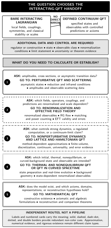
Schematic question-to-destination map for interacting QFT. A bare Lagrangian gives local classical input but does not directly define a continuum quantum theory; regulator and state choices, renormalization conditions, observables, limit statements, and evidence are additional. Five independent routes send scattering, scale-dependent observables, nonperturbative or lattice evidence, state or background questions, and existence theorems to their developed treatments. The cards are alternatives selected by the question, not stages in one construction.

The table reproduces every route without relying on the figure.

Interacting-QFT questions and the object each developed treatment controls

Requested output	Object and control data	Continue to	Do not infer
Amplitudes or asymptotic transitions	In/out states, normalization, infrared prescription, perturbative order, and uncertainty	Scattering and the Dyson series	A universal scattering sector or a convergent global Dyson operator
Running, matching, and effective operators	Renormalized observable, scheme, scale, operator basis, power counting, and truncation	Renormalization and effective field theory	That a field coordinate or coefficient is regulator-independent by itself
Nonperturbative continuum approximation	Hierarchy, regulator, truncation or closure, state, symmetry constraints, and benchmarks	Nonperturbative functional equations	That a truncated solution proves existence, uniqueness, or exactness
Lattice continuum evidence	Action, tuned trajectory, operator matching, ensembles, extrapolation, and errors	Lines of constant physics and continuum extrapolation	That several finite-spacing results already define the continuum theory
Thermal or nonequilibrium state observables	Initial state (or density operator when available), contour, measured operators, conservation laws, and approximation range	Thermal and nonequilibrium QFT	Vacuum or in/out assumptions in a general initial-state problem
Fields and states on curved backgrounds	Geometry, state class, local covariance, renormalization freedom, and backreaction regime	QFT in curved spacetime	A preferred global particle or vacuum representation
Existence, axioms, representations, or reconstruction	Exact object class, domains, topology, state, axioms, and limiting family	Mathematical-QFT construction claims	That perturbative or numerical evidence has silently become a theorem

For the formal local construction mentioned above, the precise downstream worked examples are The Perturbative AQFT Bogoliubov Map and Adiabatic Limits and Algebraic Interacting Nets. They develop the theorem-level hypotheses; they are not prerequisites for the physical distinctions on this page.

Common pitfalls

“The interacting propagator is just the free propagator with a shifted mass.” A pole shift is only one part of the spectral change. Residues, continua, operator mixing, contact terms, and possibly the very existence of a stable pole also matter.

“A renormalized field is an observable.” Renormalized fields and composite operators are scheme- and normalization-dependent coordinates. Physical claims should be attached to specified matrix elements, poles, cross sections, expectation values, or other matched observables.

“Free asymptotic fields restore the interaction picture.” In/out fields are large-time limits on scattering subspaces. They do not give one global unitary equality between the finite-time interacting field and a free field on the whole Hilbert space.

“A formally exact hierarchy or local S-matrix is already a nonperturbative model.” Exactness within a formal-series algebra or before a truncation is a typed statement. Convergence, a positive Hilbert-space state, regulator removal, and global existence require additional arguments.

Check your understanding

1. A scalar two-point function has an isolated pole and a continuum. Which structures are free, renormalized, and still unproved?

Answer

The free pole denominator is useful spectral language, while the physical pole mass, residue, and continuum are properties of the interacting operator and state. The pole supports a stable one-particle interpretation under the stated positivity and isolation assumptions. It does not by itself prove Haag–Ruelle scattering, wave-operator existence, or asymptotic completeness.

2. Why do Wick contractions remain useful after Haag’s theorem removes the exact global interaction picture?

Answer

They organize coefficients relative to a chosen free covariance in a regulated or formal perturbative construction. The calculation does not require the free and exact interacting fields to be globally unitarily equivalent on one continuum Hilbert space.

3. What survives a local invertible field redefinition in an effective theory?

Answer

Specified matched observables are preserved to the controlled order when the usual locality, invertibility, Jacobian, and power-counting conditions are satisfied. Individual off-shell correlators, coefficients, and the appearance of the field variable need not remain unchanged.

4. A functional-equation truncation and a lattice calculation disagree. Which route should compare them?

Answer

First compare common renormalized observables and regimes rather than bare fields. Nonperturbative QFT develops and tests the truncation, branch, and symmetry diagnostics; Lattice QFT controls tuning, finite-volume and spacing extrapolation, and statistical and systematic errors. A theorem-level existence claim goes separately to Mathematical QFT.

References

• Brunetti, Romeo, Michael Dütsch, and Klaus Fredenhagen. “Perturbative Algebraic Quantum Field Theory and the Renormalization Groups.” Advances in Theoretical and Mathematical Physics 13, no. 5 (2009): 1541–1599. DOI. Open PDF.
• Buchholz, Detlev, and Wojciech Dybalski. “Scattering in Relativistic Quantum Field Theory: Basic Concepts, Tools, and Results.” arXiv:math-ph/0509047v3, revised 2024 (originally submitted 2005). Stable record. Open PDF, v3.
• Burgess, C. P. Introduction to Effective Field Theory: Thinking Effectively about Hierarchies of Scale. Cambridge University Press, 2021. DOI.
• Dedushenko, Mykola. “Snowmass White Paper: The Quest to Define QFT.” arXiv:2203.08053v2 [hep-th], revised 2023 (originally submitted 2022). Stable record. Open PDF, v2.
• Fredenhagen, Klaus, and Katarzyna Rejzner. “Perturbative Algebraic Quantum Field Theory.” In Mathematical Aspects of Quantum Field Theories, edited by Damien Calaque and Thomas Strobl, 17–55. Mathematical Physics Studies. Springer, 2015. DOI. Open PDF, arXiv v2 revised 2013.
• Schwartz, Matthew D. Quantum Field Theory and the Standard Model. Cambridge University Press, 2014. DOI.
• Summers, Stephen J. “A Perspective on Constructive Quantum Field Theory.” arXiv:1203.3991v2 [math-ph], revised 2016 (originally submitted 2012). Stable record. Open PDF, v2.
• Wilson, Kenneth G., and John Kogut. “The Renormalization Group and the $\varepsilon$ Expansion.” Physics Reports 12, no. 2 (1974): 75–199. DOI.