Interacting QFT: Definitions, Limits, and Handoffs

Enter this chapter by asking what kind of interacting-QFT claim you need. A local interaction is important input, but it is not yet a choice of state, observable algebra, regulator, renormalization conditions, limiting procedure, or standard of error control. The first two pages separate those ingredients; the third explains the precise obstruction behind Haag’s theorem; the fourth identifies which free-field structures survive as renormalized, effective, algebraic, lattice, constructive, or asymptotic objects. From there, the desired output—not the Lagrangian by itself—selects the next volume.

From a local interaction to a controlled QFT claim

An interacting action can specify classical equations, local couplings, field content, and symmetries. It does not automatically produce a Hilbert-space theory, a probability measure, a state, composite operators, or a regulator-independent family of observables. Those objects require a declared construction and hypotheses appropriate to it. This distinction is common to canonical, Euclidean, algebraic, constructive, lattice, effective, and perturbative formulations, although the intermediate objects are not identical across those frameworks Schwartz 2014, §§ 14.2–14.4, printed pp. 254–266; § 15.4, printed pp. 296–298; and § 16.1, printed pp. 302–303, Hollands and Wald 2015, § 1, arXiv v2 printed pp. 5–8 (PDF), Summers 2016, §§ 1 and 3, printed pp. 1–4 and 9–18 (PDF).

It helps to distinguish four levels of statement:

1. Formal local input: a field list, action or interaction functional, symmetry, and classical stability conditions.
2. Regulated or formal construction: a finite lattice, momentum cutoff, finite volume, operator truncation, or a formal power series with a renormalization prescription.
3. Controlled observables: specified states and observables, normalization and renormalization conditions, an approximation or convergence statement, and an error criterion.
4. Continuum or exact claim: a declared limit or nonperturbative object, a topology or observable class in which it exists, and the structural properties actually established.

These levels are a diagnostic, not a universal linear pipeline. A useful effective field theory may deliberately retain a finite cutoff. Perturbative algebraic QFT can define local observables rigorously as formal series without asserting convergence to complex numbers. A constructive or lattice program instead faces model-specific existence and limit questions Fredenhagen and Rejzner 2015, §§ 5–7, arXiv v2 printed pp. 21–34 (PDF), Summers 2016, § 7, printed pp. 45–47 (PDF).

Check your entry point

The overview itself has no prerequisite. Each route below names the preparation its first technical step actually uses.

Preparation for the four chapter routes

Goal	Enter at	Preparation used there	If unsure: repair
Test what an interaction specifies	What an Interacting Lagrangian Does and Does Not Specify	Hard: the action principle and field equations.	Review Wick's theorem and free Gaussian factorization for the later perturbative contrast.
Evaluate a continuum-limit claim	Read page 1, then Regulators, Cutoffs, and Continuum Limits	Hard: page 1 and regulated bosonic field integrals.	Repair the analysis language with limits and completeness and Lebesgue convergence.
Understand Haag's theorem	Read page 2, then Haag's Theorem: Physical Meaning and Scope	Hard: page 2, Fock space, and Hilbert positivity and unitary evolution.	Use the canonical–functional crosswalk for regulated systems if equal-time and functional descriptions are being conflated.
Choose an interacting framework	Read pages 2 and 3, then Interacting Fields, Asymptotic Observables, and Effective Descriptions	Hard: pages 2 and 3 plus the one-particle-irreducible effective action.	Review the one-particle pole and scattering handoff if particle language is the sticking point.

If the analysis language itself is the obstacle, review Limits, Completeness, and Convergence or Lebesgue Integration and Convergence Theorems before making a regulator-removal claim.

Choose a route

Start with the Lagrangian reality check when the question is whether a classical interaction, a formal path integral, or a bounded-below potential already defines the quantum theory. The first page inventories what is fixed and what remains to be supplied.

Start with regulators and limits when a calculation already has a cutoff and the question is what must converge, what is tuned, what counts as universality, or what uncertainty remains. This route distinguishes a finite-regulator result from evidence for a target continuum theory.

Take the Haag route when an interaction picture seems to identify free and interacting fields by one global unitary transformation. The theorem page states the covariance, vacuum, irreducibility, equal-time, representation, and domain assumptions before drawing its conclusion.

Take the framework handoff when the practical question is which notion of field or observable to use. The final page compares regulated perturbation, effective descriptions, lattice observables, nonperturbative approximations, constructive models, local algebras, and asymptotic particle observables without treating them as interchangeable.

Questions determine the downstream method

The map below begins with the information that a formal interaction still lacks. Inspect the central checklist before following a branch: every destination expects a different output and a different kind of control.

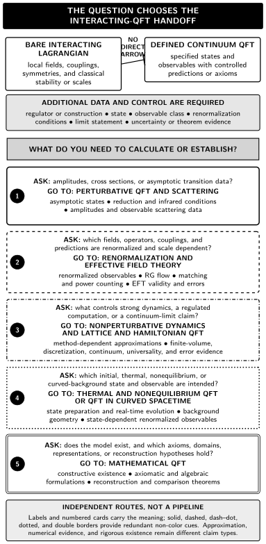
Schematic question-to-destination map for interacting QFT. A bare Lagrangian gives local classical input but does not directly define a continuum quantum theory; regulator and state choices, renormalization conditions, observables, limit statements, and evidence are additional. Five independent routes send scattering, scale-dependent observables, nonperturbative or lattice evidence, state or background questions, and existence theorems to their developed treatments. The cards are alternatives selected by the question, not stages in one construction.

The following table is the complete semantic counterpart of the figure.

Requested interacting-QFT outputs and their developed treatments

Requested output	Data that must be fixed	Control question	Continue to
Amplitudes, cross sections, or decay rates	Asymptotic states, interaction prescription, normalization, and measured parameters	Perturbative order, infrared treatment, unitarity, and uncertainty	Scattering and the Dyson series
Renormalized correlators, operators, or effective couplings	Regulator or scheme, renormalization conditions, scale, state, and observable	Scheme consistency, power counting, running, matching, and truncation error	Renormalization and effective field theory
Continuum estimates from a lattice regulator	Action, lattice spacing, volume, tuned trajectory, operators, and ensembles	Scaling window, finite-volume effects, continuum extrapolation, and uncertainty	Lattice continuum inference
Nonperturbative continuum approximation	State or vacuum, truncation, regulator, closure ansatz, and observables	Symmetry preservation, regulator dependence, convergence, and benchmark error	Nonperturbative functional equations
Thermal or real-time nonequilibrium observables	Initial density operator, contour, environment assumptions, and measured operators	Normalization, causality, conservation, equilibration, and approximation range	Thermal and nonequilibrium QFT
Fields and states on curved backgrounds	Background geometry, state class, local observables, and covariance prescription	Local covariance, renormalization freedom, state dependence, and backreaction regime	QFT in curved spacetime
Existence, reconstruction, or theorem-level continuum claims	Exact object class, topology, axioms, state, domains, and limiting family	Existence, uniqueness, positivity, locality, covariance, and proved convergence	Mathematical-QFT construction claims

The four pages in order

1. What an Interacting Lagrangian Does and Does Not Specify separates classical local input from state, regulator, observable, renormalization, and continuum data. Its hard preparation is the action principle. Its first test is a scalar quartic interaction whose classical potential is bounded below but whose continuum quantum theory is not thereby defined.
2. Regulators, Cutoffs, and Continuum Limits follows a cutoff scalar model from bare input to finite-regulator observables, tuning, convergence, universality, and error control. It requires page 1 and regulated bosonic field integrals and distinguishes numerical or perturbative evidence from a proved limit.
3. Haag’s Theorem: Physical Meaning and Scope requires page 2, Fock space, and Hilbert positivity. It states the theorem with its representation and domain hypotheses visible, then diagnoses what finite volume, regulators, perturbative constructions, and asymptotic fields change; it does not use the theorem as a slogan that perturbation theory is inconsistent.
4. Interacting Fields, Asymptotic Observables, and Effective Descriptions requires pages 2 and 3 plus the one-particle-irreducible effective action. It closes the Foundations volume by classifying free-scalar structures as retained, renormalized, replaced, framework-dependent, or merely asymptotic after interactions are introduced.

The interacting scalar reality check

Use a real scalar as the recurring comparison, with formal classical density

$$\mathcal L =\frac12\,\partial_\mu\phi\,\partial^\mu\phi -\frac12 m_0^2\phi^2 -\frac{\lambda_0}{4!}\phi^4, \qquad \lambda_0>0.$$

The potential

$$V(\phi)=\frac12m_0^2\phi^2+\frac{\lambda_0}{4!}\phi^4$$

is bounded below for the displayed quartic sign. It is not a bounded function, and bounded-below classical energy is not a construction theorem. The density fixes a classical equation and some symmetry data. It does not, by itself, decide whether the quantum object is a cutoff Hamiltonian, a Euclidean measure, a formal perturbative algebra, a lattice family, an effective theory, or a nonperturbative continuum model.

A regulator-dependent result can be denoted schematically by

$$Q_{\mathcal R} \!\left[O;\Lambda,L,\mathbf g_0(\Lambda),\rho_{\Lambda,L}\right],$$

where $O$ is the observable, $\rho_{\Lambda,L}$ the state data, $\mathbf g_0$ the bare parameters or tuning data, and $\mathcal R$ the construction. A continuum claim must say which quantities are held fixed, which limits are taken, and in what sense the observable family converges. Writing

$$Q[O] =\lim_{\substack{\Lambda\to\infty\\L\to\infty}} Q_{\mathcal R} \!\left[O;\Lambda,L,\mathbf g_0(\Lambda),\rho_{\Lambda,L}\right]$$

names a question; it does not prove that the limit exists, is unique, is regulator-independent, or has controlled errors. Nor does every legitimate framework formulate its result through this literal double limit. The four pages keep the physical observable fixed while explaining what each construction must add.

Convention and claim checklist

The same symbol can change meaning when a discussion moves from a formal density to a regulated calculation or a renormalized prediction. Keep the following distinctions visible.

• Bare and renormalized quantities: write bare parameters as $m_0$, $\lambda_0$, or with an explicit regulator label when useful. A renormalized mass or coupling such as $m_R(\mu)$ or $\lambda_R(\mu)$ is defined by stated conditions at a scale $\mu$; it is not obtained by silently relabeling a bare coefficient.
• Regulated and formal-series meanings: a cutoff expression is an ordinary object only within its finite-regulator construction. A perturbative series is usually an element of a formal power-series algebra or an asymptotic expansion. Truncating after order $N$ needs a declared remainder or uncertainty claim; it is not an exact equality merely because every displayed coefficient is finite.
• Order and topology of limits: specify whether infinite volume, regulator removal, source removal, late time, or another limit comes first. Also name the sense of convergence—of selected correlation distributions, expectation values, spectra, operator matrix elements, measures, or another object. Different orders or topologies need not agree.
• Observable comparisons: compare renormalized, dimensionless, or otherwise invariantly defined observables whenever possible. Agreement of bare coefficients, field normalizations, or regulator coordinates is not itself a universality test.

When translating between canonical and functional descriptions, first identify the finite regulated system and the same observable on both sides. The canonical–functional crosswalk supplies that bridge; it does not license an unregulated equivalence by notation alone.

What this chapter establishes

By the end of the chapter, you should be able to make four disciplined distinctions:

• Input versus construction: an action or Hamiltonian density is not the same object as a regulated theory, a formal algebra, or a continuum model.
• Finite-regulator result versus limiting claim: a stable computation at several cutoffs is evidence whose strength depends on tuning, scaling, error estimates, and the observable class.
• Theorem obstruction versus practical method: Haag’s theorem rules out a specific global interaction-picture identification under its hypotheses; it does not erase perturbative, regulated, local, or asymptotic constructions.
• Free-field language versus interacting meaning: poles, fields, particles, creation operators, propagators, and effective actions survive only with the qualifications appropriate to the chosen framework and regime.

Misconception clinic

“The quartic potential is stable, so the quantum theory exists.” Stability is important, but the state space or measure, regulator, composite operators, renormalization conditions, and limiting argument remain unspecified.

“Removing a cutoff means setting it to infinity in the last formula.” Bare data usually have to vary with the regulator, while renormalized observables and scales are held fixed. Convergence and error control must be stated in an observable class and topology.

“Haag’s theorem proves that perturbation theory is inconsistent.” It obstructs a global unitary interaction picture under a precise package of assumptions. Regulators, local perturbative constructions, switching procedures, and asymptotic fields change that package in identifiable ways.

“A common Lagrangian makes two constructions equivalent.” Matching local input or finitely many observables is not yet equivalence, universality, or uniqueness of a continuum theory. The comparison must name the objects and the relation being claimed.

“Effective or asymptotic objects are merely fake fields.” They are controlled physical descriptions when their regime, matching conditions, observables, and errors are stated. Their meaning is different from an exact global Heisenberg field, not automatically inferior.

Review the chapter

1. Retrieval — What additional data would you request after seeing only the scalar quartic density above?

Answer

At minimum: the construction or regulator, state or boundary conditions, observables, bare and renormalized parameters, normalization and renormalization conditions, limiting or formal-series meaning, and the intended error or existence claim. The precise list depends on the framework.

2. Failure diagnosis — A lattice calculation gives the same dimensionless ratio at three lattice spacings. Has it defined the continuum theory?

Answer

Not yet. The agreement is evidence. One must identify a line of constant physics, control finite-volume and discretization effects, justify the extrapolation, and state uncertainty. A construction theorem would require still stronger, explicitly named convergence and structural results.

3. Transfer — Which route should answer whether a free-particle pole survives as an interacting asymptotic state?

Answer

Use the final synthesis page to identify the spectral and asymptotic qualifications, then continue to Scattering for the developed in/out-state treatment. The existence of an isolated pole, stable particle, and asymptotic completeness are separate claims.

4. Explanation — Why does $\lambda_0>0$ not establish an interacting continuum QFT?

Answer

It proves a classical large-field stability property of the displayed potential. It does not construct the quantum state space or measure, define products of continuum fields, select renormalized observables, prove self-adjoint dynamics, or establish the regulator and volume limits.

5. Derivation and proof review — A paper writes a formal cutoff-removal limit. What must its argument establish beyond writing the limit symbol?

Answer

It must define the regulated family and tuning trajectory, identify the observables and fixed physical data, state the order and topology of limits, prove or quantitatively support convergence, control errors, and verify whichever structural properties are claimed for the limit. A formula naming the limit supplies none of those steps by itself.

6. Convention or representation change — How should a canonical cutoff Hamiltonian be compared with a Euclidean regulated measure?

Answer

Begin with a common finite regulated system and match the same observables, parameters, boundary or state data, and normalization. Then prove the appropriate transform or transfer relation. Do not identify integration variables with operators or infer an unregulated equivalence merely because the formal actions look alike.

7. Comparison — How does a finite-cutoff effective theory differ from a proposed cutoff-free continuum construction?

Answer

The effective theory treats the cutoff and operator expansion as part of a controlled finite-domain description, with matching and truncation errors. A cutoff-free construction claims that a specified family converges as the regulator is removed and must state the topology, tuned data, limiting observables, and structural properties. Neither claim is automatically stronger for every physical question; they answer different questions.

8. Synthesis — A two-loop calculation is finite after counterterms and agrees with data. What has been established, and where should the remaining questions go?

Answer

It establishes a renormalized perturbative prediction to a stated order, provided the input scheme, parameters, observable, and uncertainties are specified. Higher-order and effective-description questions go to Renormalization and EFT; amplitude and asymptotic-state details go to Scattering; convergence or nonperturbative existence goes to Nonperturbative, Lattice, or Mathematical QFT according to the object being claimed.

Where to continue

• For amplitudes and asymptotic states, continue to Scattering and the Dyson series.
• For regulator removal, renormalized predictions, running, and effective operators, continue to Renormalization and Effective Field Theory.
• For numerical continuum inference, continue to Lines of Constant Physics and Continuum Extrapolation.
• For proof-level Haag analysis, continue to Haag’s Theorem and Inequivalent Representations.
• For existence, reconstruction, and continuum-claim grammar, continue to Existence, Construction, Reconstruction, and Continuum Claims.

References

• Fredenhagen, Klaus, and Katarzyna Rejzner. “Perturbative Algebraic Quantum Field Theory.” In Mathematical Aspects of Quantum Field Theories, edited by Damien Calaque and Thomas Strobl, 17–55. Mathematical Physics Studies. Springer, 2015. DOI. Open PDF, arXiv:1208.1428v2, revised 2013.
• Hollands, Stefan, and Robert M. Wald. “Quantum Fields in Curved Spacetime.” Physics Reports 574 (2015): 1–35. DOI. Open PDF, arXiv:1401.2026v2.
• Schwartz, Matthew D. Quantum Field Theory and the Standard Model. Cambridge University Press, 2014. DOI.
• Summers, Stephen J. “A Perspective on Constructive Quantum Field Theory.” arXiv:1203.3991v2 [math-ph], revised 2016 (originally submitted 2012). Stable record. Open PDF, v2.