Maxwell Constraints as a Worked Application

Free Maxwell theory is the first field-theory example in which a singular Legendre map, constraint stabilization, and a gauge quotient can all be followed explicitly. The absent velocity $\dot A_0$ gives the primary constraint $\pi^0\approx0$; preserving it gives Gauss law as a secondary constraint; and the two first-class constraints organize one spacetime gauge function. After imposing the constraints and quotienting the admitted gauge directions, the physical initial data are one transverse canonical pair, with two configuration-space polarizations.

This page performs only that source-free Maxwell calculation on a fixed time slice in four-dimensional Minkowski space. It assumes regular fields and boundary data for which the displayed Hamiltonians and generators are differentiable. Boundary charges, harmonic and topological sectors, general constraint theory, gauge-generator algorithms, BRST/BV, and quantization are kept outside the calculation.

Required background. Hamiltonian Initial Data and Phase Space supplies canonical momenta, degenerate Legendre maps, equal-time Poisson brackets, and Hamiltonian evolution. The Free Maxwell Field and Gauge Redundancy supplies the action, field strength, equations, Gauss law, and Abelian gauge equivalence.

Helpful background. Constraints, Dirac Brackets, and Symplectic Reduction supplies the reusable first-/second-class and quotient framework.

The Maxwell Legendre map has one null velocity

Take the spatial slice to be $\Sigma=\mathbb R^3$. Fields and their variations fall off rapidly enough that the spatial surface terms displayed below vanish, and admitted gauge parameters are compactly supported or obey the corresponding vanishing condition. These assumptions also exclude harmonic and zero-mode sectors when the transverse decomposition is used later. Spatial contractions use $\delta_{ij}$.

Keep the lower components $A_\mu=(A_0,A_i)$ as the canonical coordinates throughout. With

$$\begin{aligned} F_{0i}&=\dot A_i-\partial_iA_0, \\ \mathcal L_{\mathrm M} &=\frac12F_{0i}F_{0i} -\frac14F_{ij}F_{ij}, \end{aligned}$$

the momenta are

$$\begin{aligned} \pi^\nu &\equiv \frac{\partial\mathcal L_{\mathrm M}} {\partial\dot A_\nu} =-F^{0\nu}, \\ \pi^0&=0, \qquad \pi^i=F_{0i}=E_i. \end{aligned}$$

The velocity Hessian in the order $(A_0,A_i)$ is therefore

$$W^{\mu\nu} = \frac{\partial^2\mathcal L_{\mathrm M}} {\partial\dot A_\mu\partial\dot A_\nu} = \begin{pmatrix} 0&0\\ 0&\delta^{ij} \end{pmatrix}.$$

Its rank is three. The spatial velocities are recovered as

$$\dot A_i=\pi_i+\partial_iA_0,$$

but no equation recovers $\dot A_0$. The image of the Legendre map is instead restricted by the primary constraint

$$\phi_1(\mathbf x)=\pi^0(\mathbf x)\approx0.$$

Here $\approx$ denotes equality after restriction to the final constraint surface; brackets must be evaluated before making that restriction. The electromagnetic momenta and primary relation are derived in Weinberg 1995, § 8.2, pp. 344–345. The general singular-Lagrangian step is worked in Brown 2022, § IV, p. 5.

The canonical Hamiltonian makes A₀ a multiplier

Using only the three invertible velocities gives

$$\mathcal H_c =\frac12\pi^i\pi_i +\frac14F_{ij}F_{ij} +\pi^i\partial_iA_0.$$

The final term must not be integrated by parts silently. Before the boundary assumption is imposed,

$$\begin{aligned} H_c ={}&\int_\Sigma\mathrm d^3x\, \left( \frac12\boldsymbol\pi^2 +\frac14F_{ij}F_{ij} -A_0\,\partial_i\pi^i \right) \\ &+\int_{\partial\Sigma}\mathrm dS\, A_0n_i\pi^i. \end{aligned}$$

Under the declared falloff the surface integral vanishes. Define

$$\mathcal G(\mathbf x) \equiv\partial_i\pi^i(\mathbf x),$$

and add an arbitrary multiplier $u(t,\mathbf x)$ for the primary constraint:

$$\begin{aligned} H_T&=\int_\Sigma\mathrm d^3x\, \mathcal H_T, \\ \mathcal H_T &=\frac12\boldsymbol\pi^2 +\frac14F_{ij}F_{ij} -A_0\mathcal G +u\pi^0. \end{aligned}$$

Thus $A_0$ and $u$ play different roles. The field $A_0$ already occurs in the canonical Hamiltonian as the multiplier of Gauss law, whereas $u$ is the undetermined velocity $\dot A_0$ introduced with the primary constraint.

Stabilization produces Gauss law and then closes

Use the equal-time bracket

$$\begin{aligned} \{F,G\} ={}&\int_\Sigma\mathrm d^3x\, \frac{\delta F}{\delta A_\mu} \frac{\delta G}{\delta\pi^\mu} \\ &-\int_\Sigma\mathrm d^3x\, \frac{\delta F}{\delta\pi^\mu} \frac{\delta G}{\delta A_\mu}. \end{aligned}$$

Equivalently, the fundamental bracket is

$$\{A_\mu(\mathbf x),\pi^\nu(\mathbf y)\} =\delta_\mu{}^\nu \delta^{(3)}(\mathbf x-\mathbf y).$$

The primary constraint must hold at every time. Its Hamiltonian derivative is

$$\dot\pi^0(\mathbf x) =\{\pi^0(\mathbf x),H_T\} =\mathcal G(\mathbf x) \approx0.$$

Hence

$$\phi_2(\mathbf x) =\mathcal G(\mathbf x) =\partial_i\pi^i(\mathbf x) \approx0$$

is the secondary constraint. Because $\pi^i=E_i$, it is precisely source-free Gauss law. Its preservation gives

$$\dot{\mathcal G} =\partial_i\dot\pi^i =\partial_i\partial_jF_{ji} =0,$$

where the last equality follows from the antisymmetry of $F_{ji}$. There is no tertiary constraint, and no consistency equation fixes $u$.

For a distributionally safe classification, smear both constraints with admissible test functions. All three brackets vanish strongly:

$$\begin{aligned} \{\pi^0[f],\pi^0[g]\}&=0, \\ \{\pi^0[f],\mathcal G[g]\}&=0, \\ \{\mathcal G[f],\mathcal G[g]\}&=0. \end{aligned}$$

Both constraints are therefore first class. This conclusion uses the stabilized set and its bracket algebra, not merely the singular Hessian. Weinberg 1995, § 8.2, pp. 344–345 gives the Maxwell primary and Gauss constraints, their first-class character, and preservation of Gauss law. Brown 2022, §§ VI–X, pp. 6–11, PDF develops the general stabilization and classification steps used here in a finite-dimensional model.

Hamilton’s equations provide an independent sign check:

$$\begin{aligned} \dot A_0&=u, &\dot\pi^0&=\partial_i\pi^i, \\ \dot A_i&=\pi_i+\partial_iA_0, &\dot\pi^i&=\partial_jF_{ji}. \end{aligned}$$

The first spatial equation recovers $\pi^i=F_{0i}$. The second is the source-free Ampère equation, and its divergence reproduces preservation of Gauss law.

One gauge function links the two constraints

The Gauss constraint alone generates the spatial part of a gauge transformation. With

$$G_{\mathrm{sp}}[\alpha] =-\int_\Sigma\mathrm d^3x\, \alpha\mathcal G,$$

integration by parts gives

$$\delta_\alpha A_i =\{A_i,G_{\mathrm{sp}}[\alpha]\} =\partial_i\alpha, \qquad \delta_\alpha A_0=0.$$

For time-dependent $\alpha$, this slice transformation alone is not the full spacetime transformation: it omits the change of $A_0$. The primary constraint supplies the complementary instantaneous flow. If

$$P[\beta] =\int_\Sigma\mathrm d^3x\, \beta\pi^0,$$

then

$$\begin{aligned} \{A_0,P[\beta]\}&=\beta, &\{A_i,P[\beta]\}&=0, \\ \{\pi^\mu,P[\beta]\}&=0. \end{aligned}$$

These are not two unrelated gauge symmetries. To match the Lagrangian redundancy $\delta_\alpha A_\mu=\partial_\mu\alpha$, their descriptors are tied by $\beta=\dot\alpha$: the value of one function $\alpha(t,\mathbf x)$ controls the longitudinal spatial shift, and its first time derivative controls $A_0$ on the same slice. The general construction of the tuned generator, including its action on multipliers, belongs to Gauge Orbits, Gauss Constraints, and Stabilizers.

Zinn-Justin 2021, § 21.5.2, p. 518 independently exhibits the Gauss constraint as the generator of the residual spatial transformation after temporal gauge has been chosen. That restricted statement supports $G_{\mathrm{sp}}$ above; the relation to the four-component Lagrangian transformation is supplied by the linked instantaneous flows and $\beta=\dot\alpha$, while the general tuned-generator construction is handed off.

The constraint surface also makes the gauge direction geometrically visible. Pull back the canonical two-form

$$\Omega_\Sigma =\int_\Sigma\mathrm d^3x\, \left( \boldsymbol\delta A_0\wedge\boldsymbol\delta\pi^0 +\boldsymbol\delta A_i\wedge\boldsymbol\delta\pi^i \right).$$

For a tangent variation, $\boldsymbol\delta\pi^0=0$ and $\partial_i\boldsymbol\delta\pi^i=0$. Contracting $\Omega_\Sigma$ with the gauge vector gives a term proportional to

$$\int_\Sigma\mathrm d^3x\, \partial_i\alpha\, \boldsymbol\delta\pi^i =-\int_\Sigma\mathrm d^3x\, \alpha\,\partial_i\boldsymbol\delta\pi^i =0,$$

where the boundary term vanishes by assumption. The admitted gauge flow is therefore a null direction of the pulled-back two-form. General conditions for turning such null leaves into a smooth quotient remain with Mathematical Methods.

The complete chain is summarized below. Read it from the degenerate Legendre map through stabilization, then inspect how the primary flow controls $A_0$ and the Gauss flow controls the longitudinal part of $A_i$ before the transverse quotient.

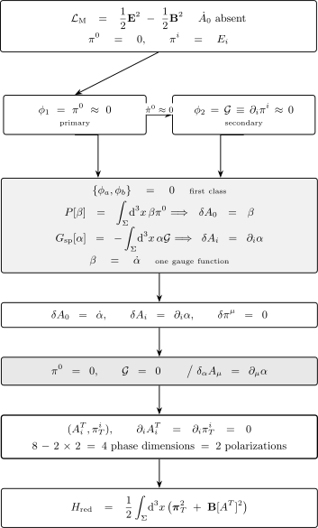
Schematic Maxwell constraint flow on $\mathbb R^3$ with the stated falloff and no harmonic or zero modes. The primary constraint $\pi^0\approx0$ stabilizes to $\mathcal G=\partial_i\pi^i\approx0$, and both are first class. The primary flow changes $A_0$ while the Gauss flow changes the longitudinal part of $A_i$; matching the covariant redundancy ties their descriptors by $\beta=\dot\alpha$. Imposing the constraints and quotienting this admitted gauge direction leaves $(A_i^T,\pi_T^i)$: four phase-space dimensions, or two configuration-space polarizations, per nonzero momentum mode. The diagram is not to scale.

Reduction leaves transverse initial data

Under the stated assumptions, decompose the spatial canonical variables as

$$\begin{aligned} A_i&=A_i^T+\partial_i\chi, &\partial_iA_i^T&=0, \\ \pi^i&=\pi_T^i+\partial^i\sigma, &\partial_i\pi_T^i&=0. \end{aligned}$$

Gauss law becomes $\nabla^2\sigma=0$. With the harmonic and zero modes excluded, $\sigma=0$, so the momentum is transverse. The gauge transformation shifts $\chi\mapsto\chi+\alpha$ and leaves $A_i^T$ unchanged. The primary constraint removes $\pi^0$, its gauge direction removes $A_0$, Gauss law removes the longitudinal momentum, and the spatial gauge quotient removes the longitudinal potential. The reduced data are therefore

$$(A_i^T,\pi_T^i), \qquad \partial_iA_i^T =\partial_i\pi_T^i =0.$$

The local dimension count says the same thing:

$$\underbrace{8}_{A_\mu,\pi^\mu} -2\times \underbrace{2}_{\text{first-class constraints}} =4$$

phase-space dimensions remain, hence two canonical pairs and two configuration-space polarizations. This count assumes independent, constant-rank constraints and a regular gauge quotient; it is not a theorem about boundary, topological, or zero-mode sectors.

The reduced Hamiltonian is

$$H_{\mathrm{red}} =\frac12\int_\Sigma\mathrm d^3x\, \left( \boldsymbol\pi_T^2 +\mathbf B[A^T]^2 \right).$$

It is positive and contains no $A_0$ or longitudinal data. For nonzero spatial momentum, the induced classical bracket is the transverse projector

$$\begin{aligned} \{A_i^T(\mathbf x),\pi_T^j(\mathbf y)\} &=\mathsf P_i{}^j \delta^{(3)}(\mathbf x-\mathbf y), \\ \mathsf P_i{}^j &=\delta_i{}^j -\frac{\partial_i\partial^j}{\nabla^2}. \end{aligned}$$

The inverse Laplacian makes the boundary and zero-mode assumptions visible rather than optional. Zinn-Justin 2021, § 21.5.1, p. 516 gives the transverse projector and the $d-2$ component count. Srednicki 2006, § 55, printed pp. 336–337, author manuscript gives the vanishing-at-infinity assumption, transverse canonical momentum, two polarizations, and reduced Hamiltonian in Coulomb gauge.

What this worked application establishes

The Maxwell Hamiltonian realizes the complete elementary constraint chain:

• the singular Legendre map yields the primary relation $\pi^0\approx0$;
• stabilization yields the secondary Gauss constraint $\partial_i\pi^i\approx0$;
• the closed bracket algebra makes both constraints first class;
• one linked primary–secondary chain corresponds to $A_\mu\mapsto A_\mu+\partial_\mu\alpha$; and
• restriction followed by the admitted gauge quotient leaves the transverse canonical pair and two physical polarizations.

The order matters. A primary constraint is not yet a gauge choice, a secondary constraint need not be second class, and restriction to the final constraint surface is not yet the gauge quotient.

The next canonical step is Physical-Mode Quantization of the Free Electromagnetic Field, which quantizes the transverse data rather than repeating their classical reduction. General gauge orbits, stabilizers, boundary charges, and the construction of generators belong to Gauge Orbits, Gauss Constraints, and Stabilizers; gauge fixing, ghosts, and cohomological machinery belong to Gauge Fixing, BRST, and BV.

Common pitfalls

Calling $\pi^0=0$ a gauge condition. It is a primary constraint produced by the Legendre map. A gauge condition is an additional representative choice and is not imposed in this derivation.

Inferring first class from a singular Hessian. Singularity only starts the analysis. The Proca field has the same missing $\dot A_0$ but a second-class constraint pair; Maxwell’s first-class result follows only after stabilization and bracket classification.

Using Gauss smearing as the whole spacetime transformation. $-\int\alpha\mathcal G$ gives $\delta A_i=\partial_i\alpha$ on a slice but leaves $A_0$ unchanged. The Maxwell transformation of all four potential components links this flow to the primary direction with descriptor $\dot\alpha$.

Dropping surface terms before specifying the phase space. If $\alpha$ or the canonical data have nontrivial boundary behavior, the generator may require a surface improvement and may carry a charge. Such a direction is not automatically redundancy; the boundary-sensitive interpretation belongs to Gauge Orbits, Gauss Constraints, and Stabilizers.

Applying the transverse count to zero or global modes. The inverse Laplacian and Helmholtz decomposition depend on boundary, falloff, and topology. Harmonic modes and nontrivial global sectors require a separate analysis.

Check your understanding

1. Starting from $\mathcal L_{\mathrm M}$, derive $\mathcal H_c$ before and after spatial integration by parts, including the surface term.

   Solution

   Since $\pi^i=F_{0i}$, one has $\dot A_i=\pi_i+\partial_iA_0$. Therefore

   $$\begin{aligned} \mathcal H_c &=\pi^i\dot A_i-\mathcal L_{\mathrm M} \\ &=\frac12\boldsymbol\pi^2 +\frac14F_{ij}F_{ij} +\pi^i\partial_iA_0. \end{aligned}$$

   Integrating the last term by parts gives $-\int_\Sigma A_0\partial_i\pi^i$ plus $\int_{\partial\Sigma}\mathrm dS\,A_0n_i\pi^i$. Only the declared falloff makes the latter vanish.

2. Verify the two smeared constraint flows and explain why neither one alone is the full time-dependent Maxwell transformation.

   Solution

   For the displayed $P[\beta]$, the canonical bracket gives $\delta A_0=\beta$ and $\delta A_i=0$. For the displayed $G_{\mathrm{sp}}[\alpha]$, integration by parts gives $\delta A_i=\partial_i\alpha$ and $\delta A_0=0$. Both leave $\pi^\mu$ unchanged. Neither flow alone changes all four components as a time-dependent Maxwell transformation does; matching $\delta A_\mu=\partial_\mu\alpha$ ties them by $\beta=\dot\alpha$, after which

   $$\delta F_{\mu\nu} =\partial_\mu\partial_\nu\alpha -\partial_\nu\partial_\mu\alpha =0.$$

3. For a nonzero Fourier mode with wavevector $\mathbf k$, reproduce the physical dimension count directly.

   Solution

   Decompose each spatial vector into two directions orthogonal to $\mathbf k$ and one parallel direction. Gauss law $k_i\pi^i=0$ removes the longitudinal momentum, while $\delta A_i=ik_i\alpha$ identifies the longitudinal potential. The primary constraint removes $\pi^0$, and the $\dot\alpha$ part of the gauge transformation identifies $A_0$. Two transverse components of $A_i$ and their two conjugate momenta remain: four phase-space dimensions, or two polarizations.

References

• Brown, J. David. “Singular Lagrangians, Constrained Hamiltonian Systems and Gauge Invariance: An Example of the Dirac–Bergmann Algorithm.” Universe 8, no. 3 (2022): 171. DOI.
• Srednicki, Mark. Quantum Field Theory. Author-hosted manuscript. Santa Barbara: University of California, 2006. Author’s page.
• Weinberg, Steven. The Quantum Theory of Fields. Volume I: Foundations. Cambridge: Cambridge University Press, 1995. DOI.
• Zinn-Justin, Jean. Quantum Field Theory and Critical Phenomena. 5th ed. Oxford: Oxford University Press, 2021. DOI.