

Correlators, Sources, and Effective Actions
A source does more than perturb a field equation: it packages an entire family of ordered correlation functions into one object. Taking a logarithm keeps only connected correlations, and, where the source–mean-field map is locally invertible, a Legendre transform reorganizes the same local information around the source-dependent mean field. This chapter develops that sequence as
while keeping two different statements alongside it: Wick factorization is a special property of free Gaussian fields, whereas Schwinger–Dyson identities follow from regulated changes of integration variables. Neither is another arrow in the –– sequence.
The recurring example is a regulated real scalar field in the normalized Lorentzian in–out convention. Ordering, state, boundary prescription, regulator, source sign, and normalization remain part of every claim. In particular, the ordinary in–out effective action is not automatically real or causal, and an exact Schwinger–Dyson hierarchy is not thereby a solved one.
Choose an entry route · See the information map · Review the chapter
Enter this chapter
Section titled “Enter this chapter”In four-dimensional Minkowski spacetime, let denote the field-integration cycle together with the vacuum boundary-value prescription, and write . For the source term in the action, define the normalized functional
This compact notation presupposes a regulator or another definition sufficient to make the operations meaningful. Source differentiation generates vacuum time-ordered moments,
and the logarithm generates their connected parts,
The factors of belong to this Lorentzian convention; changing the sign of the source term or moving to Euclidean signature changes them. Dividing the unnormalized functional by its zero-source value is equally consequential: it gives and removes vacuum factors from normalized correlators. The source derivation and the free Gaussian example are developed in Schwartz 2014, § 14.3, pp. 261–264; the regulated Euclidean counterpart and its normalization are given in Zinn-Justin 2021, §§ 7.1–7.2.1, pp. 126–127.
The mean field is
Where the map is locally invertible, the chapter uses
It follows that
Here and mean functional Hessians. The connected two-point function carries the additional convention-dependent factor shown above; silently using the same symbol for both objects is a common source of sign errors. At , is stationary. Interpreting that stationarity as a real causal evolution equation would require a different physical setup, such as an appropriate in–in construction. Zinn-Justin 2021, § 7.7, pp. 141–144 uses the Euclidean ordering . After both Legendre transforms have been rewritten in one common set of algebraic variables, the convention here reverses those two terms: . This comparison explains the minus signs in the stationarity and inverse-Hessian equations, but it is not the Wick-rotation relation between uncontinued Euclidean and Minkowski effective actions; analytic continuation supplies its own factors of .
Check your preparation
Section titled “Check your preparation”This overview has no prerequisite. The individual pages do. Use the repair link whenever the stated check is not yet routine.
| Try this | Ready when | Repair if unsure |
|---|---|---|
| Differentiate twice | You recover at and distinguish the full function from its logarithm | Gaussian Fields and Sources |
| Compare $D_F=\langle0 | T\phi\phi | 0\rangleG_F=iD_F$ |
| Invert the map | You obtain on the stated subspace and notice that zero modes obstruct the step | Vector Spaces, Duals, Linear Maps, and Bases |
| Integrate a total derivative in a finite-dimensional regulated integral | You retain the boundary term unless the integration domain and decay make it vanish | Changes of Variables and Regulated Jacobians |
For a guided curriculum route, Functional integrals and correlators connects the regulated Gaussian calculation to the source, propagator, and canonical descriptions. Use the readiness criteria above to identify which prerequisite or derivation needs repair.
Choose a route
Section titled “Choose a route”The chapter branches because the five pages answer different questions. Follow the route whose exit test matches the calculation you need.
| Reader goal | Required and helpful preparation | Observable exit |
|---|---|---|
| Recover ordered correlators and understand free pairings | Required: Gaussian sources → the generating functional; Wick’s theorem requires both pages. Helpful: scalar propagator taxonomy. | Derive the source factors and reconstruct a centered free bosonic -point function from two-point contractions |
| Separate connected response from one-particle-irreducible vertices | Required: the generating functional → connected correlators → the 1PI effective action. Helpful: characteristic functions and cumulants. | Move between , , and with the declared Legendre sign and verify the inverse-Hessian relation |
| Derive exact identities from field redefinitions | Required: the generating functional → Schwinger–Dyson identities. Helpful: regulated changes of variables and the 1PI effective action. | State the boundary and Jacobian assumptions, display the contact term, and distinguish an exact hierarchy from a closure or solution |
The correlator information map
Section titled “The correlator information map”The map below separates transformations of generating objects from relations that use additional input. Read the solid vertical path first. Then inspect the dashed boxes: the upper one returns only under the centered free-bosonic Gaussian hypothesis, while the lower one constrains through a regulated field shift.
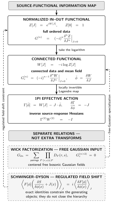
Schematic information map for the normalized Lorentzian in–out convention. Solid arrows show . Dashed return arrows mark centered free-bosonic Wick factorization and regulated Schwinger–Dyson identities as separate relations, not further transforms; the diagram is not to scale.
The figure’s relationships can be read without the image as follows.
| Object or relation | Operation and information retained | Qualification |
|---|---|---|
| Source differentiation gives all normalized ordered moments | Ordering, state, contour, normalization, and source sign are part of its definition | |
| The logarithm removes disconnected products; is the mean field | A branch of the logarithm and a neighborhood with are implicit | |
| A locally invertible source–mean-field map trades for ; its Hessian is minus the inverse of the Hessian | Zero modes and global noninvertibility require separate treatment; Euclidean convexity does not transfer automatically to in–out signature | |
| Wick factorization | A centered free bosonic Gaussian moment is a sum over products of two-point functions; connected functions above order two vanish | This is not an identity for an arbitrary interacting state or measure |
| Schwinger–Dyson relation | Regulated integration by parts relates insertions of the field equation to contact terms and produces an infinite hierarchy | Exactness does not imply closure, uniqueness, convergence, or a practical solution |
The five pages in order
Section titled “The five pages in order”The sidebar follows , pauses for the free-Gaussian Wick specialization, continues to , and finally returns to the independent Schwinger–Dyson branch. The dependency graph is not purely linear: Schwinger–Dyson identities branch directly from the generating functional.
-
The Generating Functional. Required background is Gaussian Fields and Sources; characteristic functions and cumulants are helpful. Define normalized , derive ordered source derivatives with their factors of , and keep the state, contour, boundary prescription, and zero-source normalization visible. This page is the shared entrance to every later construction.
-
Connected Correlators and Cumulants. Required background is The Generating Functional; the same cumulant methods are helpful. Pass from moments to connected functions using , derive the partition relations, and explain why connectedness is an algebraic organization rather than a claim about spatial clustering.
-
Wick’s Theorem and Free Gaussian Factorization. Required background is The Generating Functional together with Gaussian Fields and Sources; Gaussian random distributions and Wick structure are helpful. Prove the pairing rule for free Gaussian fields and track the distinct bosonic and fermionic combinatorics. Its theorem is not extended to arbitrary interacting correlators; interacting Wick expansions belong to Perturbative QFT and Scattering.
-
The 1PI Effective Action and Mean-Field Equations. Required background is Connected Correlators and Cumulants. Perform the local Legendre transform from connected to , derive the stationarity and inverse-kernel identities, and state the qualifications from zero modes, invertibility, signature, and boundary conditions. Renormalized effective actions and Wilsonian comparisons belong downstream.
-
Schwinger–Dyson Identities. Required background is The Generating Functional; the 1PI effective action and regulated changes of variables are helpful. Derive the regulated integration-by-parts identity, expose its contact terms and Jacobian assumptions, and organize the resulting exact hierarchy. Nonperturbative closures, truncations, numerical solutions, and 2PI/nPI constructions are not supplied here.
Conventions that control the hierarchy
Section titled “Conventions that control the hierarchy”The chapter inherits the site’s metric convention. The additional data below control the source hierarchy and must travel with any formula taken from it.
| Datum | Chapter convention | Check before reuse |
|---|---|---|
| Source phase | The Lorentzian weight is | One derivative of gives before normalization factors are simplified |
| Normalization | , so | Vacuum factors do not reappear in normalized moments |
| Ordering and state | The basic moments are vacuum in–out time-ordered correlators | Retarded, advanced, thermal, Euclidean, and in–in functions are not inferred from the same symbol |
| Propagator symbols | $D_F=\langle0 | T\phi\phi |
| Connected functional | and | $G_c^{(n)}=(-i)^{n-1}\delta^nW |
| Legendre sign | and | |
| Regulated field shift | Boundary terms vanish and the regulated measure and domain transform as stated | A nontrivial Jacobian, boundary contribution, or anomalous limit is retained rather than silently discarded |
The regulated free scalar as a common thread
Section titled “The regulated free scalar as a common thread”For a free scalar with the same Feynman boundary prescription in its quadratic kernel and inverse, the normalized source functional is
Because is quadratic, its derivatives above second order vanish. The full even moments generated by nevertheless do not vanish: they are sums over pairings of , while centered odd moments vanish. This is the precise free-bosonic content of Wick factorization, illustrated directly for the four-point function in Schwartz 2014, § 14.3.2, p. 263 and expressed through connected functions in Zinn-Justin 2021, § 7.3, pp. 129–131.
If on the declared regulated space, then and
Thus one regulated Gaussian exhibits the entire solid path: contains all moments, retains the connected two-point kernel, and contains its negative inverse. It also supplies the cleanest checks of the side relations. Wick’s theorem reconstructs the full moments from . For the next identity, denotes the expectation of normalized by the source-dependent functional on the same in–out cycle. Regulated integration by parts then yields, for suitable ,
The right-hand side becomes the contact term that couples different levels of the Schwinger–Dyson hierarchy. The identity assumes an adequate regulator, a domain or cycle for which the boundary contribution vanishes, and the stated behavior of the measure under the field shift. Zinn-Justin 2021, §§ 7.5–7.5.1, pp. 133–135 derives the regulated Euclidean hierarchy from the weight and distinguishes it from later approximation schemes. Replacing that weight by makes differentiation of the exponent produce , which gives the displayed Lorentzian factor and source sign.
What the five constructions say together
Section titled “What the five constructions say together”The five objects are complementary, not competing definitions of the same thing.
| Question | Construction that answers it | Category error to avoid |
|---|---|---|
| What are all ordered moments in the chosen state and prescription? | Treating normalization or the contour as dispensable decoration | |
| Which parts cannot be written as products of lower moments? | and connected correlators | Confusing algebraic connectedness with cluster decomposition at large separation |
| When do higher moments reduce to two-point data? | Wick factorization for free Gaussian fields | Applying the free pairing rule to an arbitrary interacting theory |
| What source produces a mean field, and what kernel locally inverts its response? | Assuming global invertibility, Euclidean convexity, or causal reality in the in–out problem | |
| Which exact relations follow from regulated field variations? | Schwinger–Dyson identities | Calling an infinite exact hierarchy closed or solved |
This organization also identifies the chapter boundary. Diagrammatic perturbation theory, renormalized sources and composite operators, Wilsonian coarse graining, 2PI/nPI effective actions, and nonperturbative closure schemes all use these objects but add new structure. They are developed in the respective downstream volumes.
Review the chapter
Section titled “Review the chapter”Use each success criterion to diagnose which step needs revision, then follow the corresponding repair route.
| Review mode | Prompt | A successful response | Repair route |
|---|---|---|---|
| Factor check | Derive the first two source derivatives for | Recovers $G^{(1)}=\delta W/\delta J | _0G_c^{(2)}=-iW^{(2)} |
| Gaussian synthesis | Start from | Shows that connected derivatives above order two vanish while full even moments remain as pairings of | Wick’s Theorem |
| Legendre check | Differentiate while | Obtains and the Hessian product , with an invertibility qualification | The 1PI Effective Action |
| Identity diagnosis | Explain every assumption behind the displayed Schwinger–Dyson relation | Names the regulator, integration domain or cycle, vanishing boundary term, measure or Jacobian behavior, and contact term | Schwinger–Dyson Identities |
| Formulation boundary | Decide whether an in–out gives a real causal equation for expectation values | Says “not in general,” identifies the state and contour mismatch, and routes causal evolution to an in–in construction | Lorentzian, Euclidean, and In-In Formulations |
| Convention translation | Compare with the site’s , then discuss continuation | First rewrites both Legendre transforms in common algebraic variables, identifies the reversed-term sign, and then treats Euclidean–Minkowski analytic continuation as a separate step carrying its own factors of | The 1PI Effective Action |
| Bounded transfer | For symmetric invertible matrix and , construct , , and | Obtains , , , and states what fails if has a zero mode | Connected Correlators → The 1PI Effective Action |
Where to go next
Section titled “Where to go next”- Interpret the same data physically: States, Observables, and Spectra asks what the correlators reveal about states, spectral support, positivity, and observable content.
- Change the contour or state: Lorentzian, Euclidean, and In-In Formulations develops analytic continuation, Euclidean Schwinger functions, thermal contours, and causal closed-time-path observables; Thermal and Nonequilibrium QFT develops their many-body use.
- Turn Wick structure into diagrams: Perturbative QFT and Scattering develops interacting Wick expansions, Feynman rules, amplitudes, and cross sections.
- Renormalize the generating objects: Renormalization and Effective Field Theory develops renormalized sources, composite-operator mixing, effective actions beyond the elementary definition, and the Wilsonian comparison.
- Develop functional hierarchies: Schwinger–Dyson Hierarchies and Inputs and 2PI/nPI Effective Actions develop truncations, closures, and nonperturbative applications.
References
Section titled “References”Original QFT.org content:CC BY 4.0, unless an item supplies different terms. Third-party material retains its own terms.