

Closed-Time-Path Grammar
A closed time path turns one initial-state problem into a generating functional by evolving a ket forward, evolving its bra backward, and sewing the two histories before taking a trace. The two branches therefore carry opposite action and source signs. Contour ordering then produces four two-point functions: time ordered, anti-time ordered, greater, and lesser. Exact unitary evolution closes the construction with . The doubled fields are bookkeeping histories, not two physical copies. This page fixes that grammar at a finite regulator, assembles the free-scalar matrix for a general Gaussian initial state, and stops before Keldysh rotations, thermal identities, kinetic equations, or open-system applications.
Required background. In–Out versus In–In Expectation Values supplies the normalized trace, branch-source signs, diagonal identity , and the density-operator and regulator qualifications used here.
Helpful background. Retarded, Advanced, and Spectral Correlators supplies the site convention , its advanced counterpart, and their response interpretation.
One contour carries two branch histories
Section titled “One contour carries two branch histories”Work in a finite-volume, UV-regulated closed system with a positive Hermitian initial density operator , normalized by . The trace-class formula also applies to normal states in a chosen representation; it is not a claim that every continuum algebraic state is represented by a global density operator on vacuum Fock space. Let lie later than every insertion, and retain the site source convention
The closed-time-path functional is
The branch runs from to and the branch returns from to . At a finite field regulator, the same construction reads schematically
where . The common final field implements the sum over a complete final basis. The initial kernel closes that sum through the one specified state. These branch signs, the density kernel, and final sewing follow directly from the operator trace; see Calzetta and Hu 2008, §§ 6.3.1–6.3.2, pp. 181–186.
The figure summarizes the construction. Inspect the traversal direction, the two exponent signs, and the distinct roles of the initial kernel and final sewing.
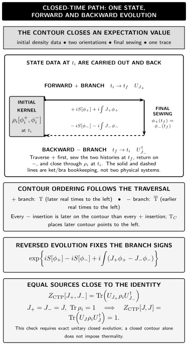
Schematic closed-time-path grammar. The ket branch evolves with , the bra branch returns with , the fields are sewn at , and the trace closes through . Later contour positions are ordered to the left. For a normalized state and exact unitary closed evolution, equal sources give . The diagram is not to scale.
The same information has the following text form.
| Contour element | Direction and ordering | Contribution or role |
|---|---|---|
| initial kernel | joins the two endpoints at | supplies |
| branch | ; ordinary time ordering | contributes |
| final sewing | identifies the two histories at | implements the final-state sum, not a postselection |
| branch | ; anti-time ordering | contributes |
| equal-source limit | aligns after differentiation | gives for exact unitary evolution |
This contour is not intrinsically thermal. Thermality would be additional information about and, in equilibrium, further analytic or KMS structure.
Source differentiation fixes the branch signs
Section titled “Source differentiation fixes the branch signs”Let and . The contour-ordering operator places later positions along the full traversal to the left. With raw correlators—no conventional prefactor of —define
The source derivatives therefore obey
For , the analogous formula gives the connected correlator:
The factors are not optional notation: they encode the minus sign on the return branch. Sources must remain independent through differentiation. Setting first reduces the functional to and erases every transverse branch variation.
Many references instead define . The component formulas below use the site’s raw convention; importing a literature matrix without removing its common changes both its normalization and its response combinations. Altland and Simons use that common alternative convention in their compact branch construction Altland and Simons 2023, §§ 12.2.1 and 12.2.4, pp. 706–707 and 716–717.
Four components follow from one contour ordering
Section titled “Four components follow from one contour ordering”Write
Every -branch point is later on the contour than every -branch point. Within the branch, contour order is ordinary time order; within the branch, it is anti-time order. Consequently,
Equivalently,
For a Hermitian real scalar and a Hermitian state,
Differentiating twice along the common-source direction gives the branch sum rule
This is the two-point form of the largest-time cancellation: an insertion on the latest real-time slice cancels when the same operator is placed on the two branches with their relative contour sign. Haehl, Loganayagam, and Rangamani derive the branch matrix, its sum rule, the trace construction, and the aligned-source cancellation in Haehl, Loganayagam, and Rangamani 2017, § 2, pp. 9–11; § 3, pp. 14 and 18.
A later review gives the trace, four-component matrix, and -point largest-time rule together in Haehl and Rangamani 2024, § 1.1, pp. 6–7 (Open manuscript PDF). Its component functions carry the conventional overall factor , and its retarded function has the opposite sign from the site convention; the raw formulas and response on this page include both translations.
At coincident times these expressions are distributional. Elementary two-point functions may use a consistent convention such as ; derivative and composite insertions can add local contact terms. The safe statement is obtained after smearing and with one consistent causal splitting on every branch.
A general Gaussian free-scalar state
Section titled “A general Gaussian free-scalar state”A finite-volume free scalar with a UV cutoff is a finite collection of real canonical modes. Put
A general Gaussian state is determined by its mean and symmetrized covariance
The last inequality is the quantum uncertainty condition. It allows mixed states, squeezing, mode correlations, and nonstationary states; Gaussianity alone does not imply a thermal occupation-number form.
For any free Heisenberg field linear in the initial canonical data,
and the centered Wightman functions are
The full functions add to both. Thus the mean and covariance carry the state dependence, while the free canonical commutator fixes their difference.
For a concrete block, take one stable real-scalar normal mode with ,
Write and . Its mean evolves as
and a general one-mode Gaussian covariance is described by
The symmetric kernel is
Define
Since ,
The required free-scalar contour matrix is therefore
with every and evaluated at . It obeys
without assuming stationarity or thermality. Calzetta and Hu give the general mixed Gaussian density matrix, its three symmetrized variances, and their free evolution in Calzetta and Hu 2008, § 4.1.6, pp. 103–104.
For the vacuum block,
so
This round trip checks every phase and normalization in the matrix. A multimode Gaussian state simply promotes the one-mode covariances to the full matrix ; cross-mode correlations must not be discarded unless homogeneity or another stated assumption diagonalizes them.
Unitarity and response test different parts of the matrix
Section titled “Unitarity and response test different parts of the matrix”The commutator combinations recover the site’s causal correlators:
For the free mode this gives
independent of and . That state independence is a property of a free canonical commutator, not a general claim about interacting spectral or response functions. The one-point mean and centered symmetric kernel together retain the Gaussian state data. A massless spatial zero mode has and is a free-particle sector rather than the oscillator vacuum displayed above; it requires separate treatment.
Several checks remain logically separate:
- tests normalized exact unitary closed evolution.
- tests branch ordering and the relative source signs.
- Hermitian conjugation tests the density operator and field adjoints.
- Retarded support tests the commutator combination, not the Feynman component alone.
- The uncertainty inequality tests whether the proposed Gaussian covariance defines a positive quantum state.
An approximation can pass one check and fail another. In particular, a truncation can preserve the four labels while violating diagonal normalization or causal response.
What the contour grammar does not supply
Section titled “What the contour grammar does not supply”- No automatic thermal state. A closed time path accepts arbitrary normalized initial data. KMS relations, imaginary-time legs, and fluctuation–dissipation identities require equilibrium input.
- No extra physical copy. The branch fields record ket and bra evolution. Their opposite action signs do not define a negative-norm sector.
- No arbitrary initial state from . The density kernel is independent boundary data; a vacuum Feynman prescription does not generate its means, covariances, or higher cumulants.
- No guarantee for reduced dynamics. After an environment is traced out, a standalone system evolution need not be unitary. Influence functionals, noise, dissipation, and trace preservation belong to the open-system treatment.
- No universal approximation theorem. Exact return-time independence and largest-time identities can be spoiled by an inconsistent regulator, truncation, or resummation.
- No complete ordering basis. A single forward–backward fold generates the four ordinary two-point components. More complicated out-of-time ordering can require additional folds.
- No silent generalization of statistics. Fermions require graded contour ordering and the corresponding exchange signs; gauge systems require physical-state or gauge-fixed qualifications.
There are restricted alternative calculations. Donath and Pajer give an in–out reformulation for nondissipative closed systems under their hypotheses, including the absence of the excluded infrared divergences; dissipative systems lie outside their result Donath and Pajer 2024, introduction, pp. 2–7, and § 2, p. 9 (Open PDF). This conditional computational route does not replace the normalized initial-state trace or change the four-component ordering identities. The scope comparison was checked against literature available through 9 August 2026.
Check your understanding
Section titled “Check your understanding”1. Recover the branch sum rule
Section titled “1. Recover the branch sum rule”Why does the displayed Gaussian matrix satisfy the unitarity identity for arbitrary and ?
Answer
The diagonal entries add to because their sign-function terms cancel. The off-diagonal entries also add to because their unsmeared commutator terms cancel. No vacuum, stationarity, or thermal assumption enters.
2. Find the response kernel
Section titled “2. Find the response kernel”Insert and into .
Answer
For , the difference is , so multiplication by gives . For , the two entries agree and the result vanishes. Hence .
3. Diagnose an alleged thermal consequence
Section titled “3. Diagnose an alleged thermal consequence”A calculation has and claims that the state must therefore satisfy KMS periodicity. What is missing?
Answer
Diagonal normalization follows from a normalized density operator and unitary closed evolution, regardless of whether the state is thermal. KMS periodicity requires an equilibrium state and additional analytic structure; it cannot be inferred from contour closure.
Where to continue
Section titled “Where to continue”Closed-Time-Path Generating Functionals in Practice is the canonical next treatment. It develops applied initial-state functionals, Keldysh bases, response and quench calculations, KMS structure, kinetic limits, and open-system uses. The static Gaussian matrix above supplies the exact benchmark needed before those computational extensions.
References
Section titled “References”-
Altland, Alexander, and Ben Simons. Condensed Matter Field Theory. 3rd ed. Cambridge University Press, 2023. DOI.
-
Calzetta, Esteban A., and Bei-Lok B. Hu. Nonequilibrium Quantum Field Theory. Cambridge Monographs on Mathematical Physics. Cambridge University Press, 2008. DOI. 2023 open-access reissue.
-
Donath, Yaniv, and Enrico Pajer. “The In-Out Formalism for In-In Correlators.” Journal of High Energy Physics 2024, no. 7 (2024): 064. DOI. Open PDF.
-
Haehl, Felix M., R. Loganayagam, and Mukund Rangamani. “Schwinger–Keldysh Formalism. Part I: BRST Symmetries and Superspace.” Journal of High Energy Physics 2017, no. 6 (2017): 069. DOI. Open PDF.
-
Haehl, Felix M., and Mukund Rangamani. “Records from the S-Matrix Marathon: Schwinger–Keldysh Formalism.” arXiv:2410.10602 (2024); published as “Schwinger–Keldysh Formalism,” in Records from the S-Matrix Marathon, Lecture Notes in Physics 1041, pp. 89–129. Springer, 2025. Book DOI. Open manuscript PDF.
Original QFT.org content:CC BY 4.0, unless an item supplies different terms. Third-party material retains its own terms.