Massive and Massless Spin-One Polarizations

For a nonzero future-directed momentum, a massive Proca polarization is an ordinary vector in the three-dimensional space orthogonal to a timelike momentum. A photon polarization also begins in a three-dimensional orthogonal space, but a null momentum lies inside its own orthogonal space and supplies a pure-gauge direction. Quotienting that direction leaves two helicities. The massive longitudinal vector grows like $p^\mu/m$ at fixed nonzero spatial momentum, so neither it nor the massive completeness tensor has a finite componentwise limit, even though transverse modes and conserved-current contractions can approach the photon result smoothly.

Required background. The Proca Field supplies the massive mass shell, equation-derived transversality, three-mode count, and longitudinal scaling. The Free Maxwell Field and Gauge Redundancy supplies the null mass shell, gauge equivalence of polarization representatives, and the two-mode quotient.

Helpful background. Bilinear and Hermitian Forms, Adjoints, and Isometries supplies Lorentz-signature orthogonality and orthonormal bases. Normal Forms, Spectra, and Projectors supplies basis-independent projector language.

A timelike momentum has three orthogonal polarizations

Work in four-dimensional Minkowski space and consider nonzero on-shell momenta, away from boundary, topology, and zero-mode complications. For a positive-frequency plane wave,

$$A^\mu(x)=\varepsilon^\mu(p)e^{-ip\cdot x},$$

the polarization vector is the coefficient $\varepsilon^\mu(p)$. Complex coefficients are convenient for helicity; a real classical field includes the corresponding complex-conjugate mode. Proca theory has no gauge equivalence among these coefficients.

Choose a massive momentum along the positive $z$-axis,

$$p_m^\mu=(E,0,0,k), \qquad E=\sqrt{k^2+m^2}, \qquad m>0,\quad k>0.$$

The three vectors

$$\begin{aligned} \varepsilon_1^\mu&=(0,1,0,0),\\ \varepsilon_2^\mu&=(0,0,1,0),\\ \varepsilon_L^\mu&=\frac1m(k,0,0,E) \end{aligned}$$

obey

$$p_m\cdot\varepsilon_\lambda=0, \qquad \varepsilon_\lambda^*\cdot\varepsilon_{\lambda'} =-\delta_{\lambda\lambda'}.$$

For the nontrivial third vector,

$$p_m\cdot\varepsilon_L =\frac{Ek-kE}{m}=0, \qquad \varepsilon_L^2 =\frac{k^2-E^2}{m^2}=-1.$$

Thus $p_m^\perp$ is a three-dimensional negative-definite space, and every one of its directions is physical. At $k=0$, where a direction $\widehat{\mathbf p}$ is undefined, the rest-frame basis $(0,\mathbf e_a)$ for $a=1,2,3$ gives the same count. Schwartz 2014, § 8.2.2, p. 117 constructs this fixed-frame basis and checks its transversality and normalization.

The basis-independent map onto $p_m^\perp$ is the mixed-index projector

$$T_m{}^\mu{}_\nu =\delta^\mu{}_\nu-\frac{p_m^\mu p_{m\nu}}{m^2}.$$

Because $p_m^2=m^2$, it satisfies

$$T_m^2=T_m, \qquad T_m p_m=0, \qquad \operatorname{tr}T_m=3.$$

Orthonormal completeness instead gives the two-lowered-index tensor

$$\begin{aligned} C^{(m)}_{\mu\nu} &\equiv \sum_{\lambda=1}^{3} \varepsilon_\mu^{(\lambda)} \varepsilon_\nu^{(\lambda)*}\\ &=-\eta_{\mu\nu} +\frac{p_{m\mu}p_{m\nu}}{m^2}. \end{aligned}$$

These objects differ by a sign after raising one index:

$$C^{(m)\mu}{}_\nu=-T_m{}^\mu{}_\nu, \qquad C^{(m)\mu}{}_\rho C^{(m)\rho}{}_\nu =-C^{(m)\mu}{}_\nu.$$

So the polarization sum itself is not an idempotent mixed-index projector. In the rest frame, $C^{(m)}_{\mu\nu}=\operatorname{diag}(0,1,1,1)$, an immediate sign and rank check. Weinberg 1995, § 5.3, pp. 210–212 derives the massive spin-one sum using a mostly-plus metric; reversing the metric changes his $\eta_{\mu\nu}+p_\mu p_\nu/m^2$ to the displayed $-\eta_{\mu\nu}+p_\mu p_\nu/m^2$, while its rank remains three.

A null momentum contains its own gauge direction

Now take

$$q^\mu=(\omega,0,0,\omega), \qquad \omega>0.$$

The source-free Maxwell equation requires $q\cdot\varepsilon=0$. A general solution therefore has the form

$$\varepsilon^\mu=(a,b,c,a).$$

Unlike the massive case, $q^2=0$ implies $q^\mu\in q^\perp$. The plane-wave gauge equivalence

$$\varepsilon^\mu\sim\varepsilon^\mu+\gamma q^\mu$$

can set $a$ to zero without changing $b$ or $c$. The physical polarization space is consequently

$$\mathcal P_q =q^\perp/\operatorname{span}\{q\}, \qquad \dim\mathcal P_q=3-1=2,$$

with convenient representatives

$$\epsilon_1^\mu=(0,1,0,0), \qquad \epsilon_2^\mu=(0,0,1,0).$$

The quotient is more than a count. If $q\cdot\varepsilon=0$, then

$$(\varepsilon+\gamma q)^* \cdot(\varepsilon+\gamma q) =\varepsilon^*\cdot\varepsilon,$$

because every additional term contains either $q^2$ or $q\cdot\varepsilon$. The Lorentz form therefore descends to a negative-definite form on $\mathcal P_q$. The field-strength amplitude

$$f_{\mu\nu} =-i(q_\mu\varepsilon_\nu-q_\nu\varepsilon_\mu)$$

is likewise unchanged by the shift. These are the invariant reasons that the $q^\mu$ direction is removed rather than counted as a third photon. Schwartz 2014, §§ 8.2.3–8.2.4, pp. 118–120 develops the pure-gauge direction, the two transverse representatives, and the three-versus-two comparison.

After complexifying the two-dimensional space, define

$$\epsilon_\pm^\mu =\frac1{\sqrt2}(0,1,\pm i,0).$$

For the active-rotation convention $R_z(\theta)\epsilon_h=e^{-ih\theta}\epsilon_h$, these have helicities $h=\pm1$. A real Maxwell field pairs each positive-frequency helicity amplitude with its complex-conjugate negative-frequency mode. This does not mean that the massless little group has one real two-dimensional irreducible representation: the two complex finite-helicity sectors are separate.

Massless completeness needs a reference vector

A covariant tensor that selects two representatives cannot be built from the null momentum alone. Indeed, a mixed tensor made only from $\delta^\mu{}_\nu$ and $q^\mu q_\nu$ has the form $a\delta^\mu{}_\nu+bq^\mu q_\nu$. Requiring it to annihilate $q^\nu$ forces $a=0$, after which its trace is zero rather than two.

Introduce an auxiliary vector $n^\mu$ with $q\cdot n\ne0$, and choose representatives satisfying

$$q\cdot\epsilon_a=0, \qquad n\cdot\epsilon_a=0, \qquad \epsilon_a^*\!\cdot\epsilon_b=-\delta_{ab}, \qquad a=1,2.$$

The mixed-index projector onto this two-plane is

$$\begin{aligned} P_0{}^\mu{}_\nu(q,n) ={}&\delta^\mu{}_\nu -\frac{q^\mu n_\nu+n^\mu q_\nu}{q\cdot n}\\ &+\frac{n^2q^\mu q_\nu}{(q\cdot n)^2}. \end{aligned}$$

Direct contraction gives

$$P_0q=P_0n=0, \qquad P_0^2=P_0, \qquad \operatorname{tr}P_0=2.$$

Because $P_0\epsilon_a=\epsilon_a$ and the two-plane is negative definite, orthonormal completeness gives $C^{(0)\mu}{}_\nu=-P_0{}^\mu{}_\nu$. The associated polarization sum is

$$\begin{aligned} C^{(0)}_{\mu\nu}(q,n) &\equiv \sum_{a=1}^{2} \epsilon_\mu^{(a)} \epsilon_\nu^{(a)*}\\ &=-\eta_{\mu\nu} +\frac{q_\mu n_\nu+n_\mu q_\nu}{q\cdot n} -\frac{n^2q_\mu q_\nu}{(q\cdot n)^2}. \end{aligned}$$

Again $C^{(0)\mu}{}_\nu=-P_0{}^\mu{}_\nu$. For the fixed frame above and $n^\mu=(1,0,0,0)$, the lowered-index tensor is $\operatorname{diag}(0,1,1,0)$, exactly the sum of $\epsilon_1$ and $\epsilon_2$. Its spatial part is the familiar transverse sum $\delta_{ij}-\widehat q_i\widehat q_j$ derived in Srednicki 2007, § 55, p. 337.

Changing $n^\mu$ changes the representatives and adds terms containing $q_\mu$ or $q_\nu$; it does not create another physical direction. In particular, for a conserved current $q\cdot J=0$,

$$J^{*\mu}C^{(0)}_{\mu\nu}(q,n)J^\nu =-J^*\cdot J,$$

so the reference-dependent terms vanish. The formula is a completeness relation for chosen potential representatives, not a gauge-invariant tensor identity independent of auxiliary data.

The little groups encode the same distinction

The little group is the subgroup of Lorentz transformations that preserves a standard momentum. For timelike momentum it is $SO(3)$, or $SU(2)$ on the quantum-state cover. The negative-definite space $p_m^\perp$ carries the three-dimensional spin-one representation, matching the three vectors $\varepsilon_1,\varepsilon_2,\varepsilon_L$.

For nonzero null momentum the little group is $ISO(2)$. In a finite-helicity representation its translation-like subgroup acts trivially on physical states; on potential representatives, the corresponding action can appear as a shift proportional to $q^\mu$, precisely the gauge direction quotiented above. Schwartz 2014, § 8.4.2, pp. 126–128 exhibits this little-group shift of the potential and its gauge interpretation. The remaining rotation labels the one-dimensional complex helicity classes $h=+1$ and $h=-1$. Weinberg 1995, § 2.5, pp. 68–74 derives the massive and massless little groups and the finite-helicity condition. Representations with nontrivial translation action are outside this free Proca–Maxwell comparison.

The schematic makes the change in physical polarization space visible: inspect the dashed null direction and the different projector traces, then compare the fixed-momentum limit at the bottom.

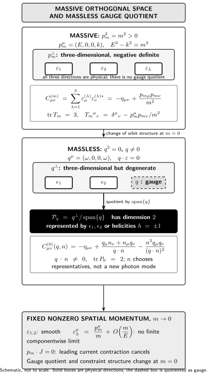
Schematic, not to scale. For $p_m^2=m^2>0$, all three directions in $p_m^\perp$ are physical and $\operatorname{tr}T_m=3$. For $q^2=0$, the direction $q^\mu$ lies inside $q^\perp$ but is pure gauge, so $q^\perp/\operatorname{span}\{q\}$ has dimension two and $\operatorname{tr}P_0=2$. The displayed completeness tensors have both indices lowered and become the negatives of the corresponding mixed-index projectors after raising one index. The limit statement assumes a fixed nonzero spatial momentum and, for current decoupling, $p_m\cdot J=0$.

The massless limit is conditional

Follow an on-shell family with fixed $\mathbf p=k\widehat{\mathbf p}$, $k>0$, and

$$p_m^\mu=(E_m,k\widehat{\mathbf p}), \qquad E_m=\sqrt{k^2+m^2}.$$

The normalized longitudinal vector obeys the exact identity

$$\begin{aligned} \varepsilon_L^\mu &=\frac1m(k,E_m\widehat{\mathbf p})\\ &=\frac{p_m^\mu}{m} +\frac{m}{E_m+k}(-1,\widehat{\mathbf p}). \end{aligned}$$

The first term diverges componentwise like $1/m$, while the second is $O(m/E_m)$. The norm nevertheless remains $-1$ because its finite value comes from cancellations among divergent components. The transverse vectors can be held fixed and have smooth limits, but $C^{(m)}_{\mu\nu}$ inherits the singular $p_{m\mu}p_{m\nu}/m^2$ term.

Now let $J_m^\mu$ be a nonsingular family of currents satisfying $p_m\cdot J_m=0$. Current conservation removes the leading term:

$$J_{m\mu}\varepsilon_L^\mu =\frac{m}{E_m+k} J_{m\mu}(-1,\widehat{\mathbf p})^\mu =O\!\left(\frac{m}{E_m}\right).$$

The full massive sum gives the sharper check

$$\begin{aligned} J_m^{*\mu}C^{(m)}_{\mu\nu}J_m^\nu &=-J_m^*\cdot J_m +\frac{|p_m\cdot J_m|^2}{m^2}\\ &=-J_m^*\cdot J_m. \end{aligned}$$

If the current and held-fixed couplings approach finite limits, this contraction can match the massless conserved-current contraction. Weinberg 1995, § 5.3, p. 212 shows the same longitudinal decoupling in a mostly-plus convention. Zinn-Justin 2021, § 21.2, p. 510 provides an independent Euclidean conserved-current check; only the algebraic current-conservation cancellation is used here, so no Euclidean polarization norm is imported.

This conditional smoothness does not identify the two state spaces. At $m=0$, a gauge quotient appears, the constraint class changes, and the longitudinal Proca state is absent from the photon spectrum. A nonconserved current, a current that itself grows as $m\to0$, or an interaction whose couplings scale singularly can retain the $1/m$ or $1/m^2$ behavior. Nor can one hold the massive rest frame fixed and reach a nonzero null momentum.

What the comparison establishes

The three-versus-two result has three mutually consistent forms:

• geometrically, $p_m^\perp$ is a three-dimensional physical space, whereas $q^\perp$ must be quotiented by its null direction;
• algebraically, the projectors have traces three and two; and
• representation-theoretically, massive spin one is an $SO(3)$ triplet while the finite-helicity photon carries the two helicity classes of the massless little group.

The spacelike Lorentz normalization $\varepsilon^*\cdot\varepsilon=-1$ is not a negative Hilbert-space norm. It records the sign of a spacelike four-vector; positivity of physical quantum states is a separate statement.

The next pages use these results in different ways. Maxwell Constraints as a Worked Application derives the two-mode count from canonical reduction. Physical-Mode Quantization of the Free Electromagnetic Field turns the two transverse representatives into photon oscillators, while Covariant Free-Photon Quantization and Propagator explains why a covariant potential description contains auxiliary components. Spinor representatives for null momenta belong to Spinor-Helicity Variables, and interacting high-energy longitudinal scattering belongs to Longitudinal Vector Bosons and the Equivalence Theorem.

Common pitfalls

Calling the lowered-index polarization sum a projector. The actual idempotent maps are $T_m{}^\mu{}_\nu$ and $P_0{}^\mu{}_\nu$. Raising one index on either polarization sum gives the negative of the corresponding projector.

Setting $m=0$ in the massive completeness relation. The term $p_\mu p_\nu/m^2$ has no such componentwise limit. Contract first with the declared observable and use current conservation only when it is genuinely available.

Counting the null momentum as a third photon. It solves $q\cdot\varepsilon=0$ because $q^2=0$, but it produces zero field strength and is removed by the gauge quotient.

Treating the reference vector as physical. The vector $n^\mu$ selects potential representatives. Conserved-current contractions eliminate its contribution; a generic gauge-dependent tensor component need not.

Check your understanding

1. Verify that $T_m^2=T_m$ and $\operatorname{tr}T_m=3$.

Solution

Write $T_m=I-p_m\otimes p_m^\flat/m^2$. Squaring produces $I-2p_m\otimes p_m^\flat/m^2+ p_m\otimes p_m^\flat(p_m^2)/m^4=T_m$. Its trace is $4-p_m^2/m^2=3$.

2. For $q^\mu=(\omega,0,0,\omega)$, show explicitly that the gauge quotient leaves two normalized representatives.

Solution

Transversality gives $\varepsilon^\mu=(a,b,c,a)$. Choosing $\gamma=-a/\omega$ sets $a$ to zero. An orthonormal basis for the remaining classes is $(0,1,0,0)$ and $(0,0,1,0)$, each with norm $-1$ and mutual inner product zero.

3. Derive the exact decomposition of $\varepsilon_L^\mu$ and test it against a conserved current.

Solution

Subtract $p_m^\mu/m$ from $(k,E_m\widehat{\mathbf p})/m$. Since $E_m-k=m^2/(E_m+k)$, the difference is $m(-1,\widehat{\mathbf p})/(E_m+k)$. Contracting with $p_m\cdot J_m=0$ removes $p_m^\mu/m$ and leaves a term of order $m/E_m$ for a nonsingular current family.

References

• Schwartz, Matthew D. Quantum Field Theory and the Standard Model. Cambridge University Press, 2014. DOI.
• Srednicki, Mark. Quantum Field Theory. Cambridge University Press, 2007. DOI.
• Weinberg, Steven. The Quantum Theory of Fields. Volume I: Foundations. Cambridge University Press, 1995. DOI.
• Zinn-Justin, Jean. Quantum Field Theory and Critical Phenomena. 5th ed. Oxford University Press, 2021. DOI.