Boundaries and State Preparation

At a fixed finite regulator, a functional integral with specified endpoint fields is a kernel, not yet an amplitude between physical states. Endpoint wave functions turn that kernel into a matrix element; one boundary integration composes two kernels; identifying the two outer endpoints and integrating once takes a trace. The same distinctions also explain how a Euclidean half-space prepares the free-scalar vacuum and why Euclidean evolution does not automatically select a unique state.

Required background. Time Slicing and Transition Amplitudes supplies the regulated kernel, endpoint normalization, ordering rule, and composition law used below.

Helpful background. Schrödinger Wave Functionals supplies configuration-space state representatives and the canonically derived free-vacuum Gaussian.

Fixed boundary fields define a kernel, not a state

Keep a spatial regulator, so a boundary field configuration is a finite vector $q=(q^1,\ldots,q^M)$. Choose configuration eigenstates and a measure $\mathrm d\mu(q)$ with compatible normalization,

$$\begin{aligned} \langle q'|q\rangle &=\delta_\mu(q'-q), \\ \mathbf 1 &=\int \mathrm d\mu(q)\,|q\rangle\langle q|. \end{aligned}$$

For ordinary Cartesian coordinates, $\mathrm d\mu(q)=\mathrm d^M q$ and $\delta_\mu$ is the $M$-dimensional Dirac delta. If a different measure is chosen, both the delta function and every resolution of the identity must change with it.

An oriented time contour $C$ from an initial boundary to a final boundary defines

$$K_C(q_f,q_i) \equiv \langle q_f|U_C|q_i\rangle.$$

Its regulated functional-integral representation has the schematic form

$$K_C(q_f,q_i) = \mathcal N_C \int_{\substack{q|_{\partial_i C}=q_i\\ q|_{\partial_f C}=q_f}} \mathcal D_C q\;e^{\,iS_C[q]},$$

with $iS_C$ replaced by $-S_E$ on a Euclidean segment. The endpoint configurations are held fixed in this expression: the path integral integrates only the interior variables. A particular value $q_i$ labels a generalized configuration eigenstate; it is not, by itself, a normalizable prepared state.

This distinction follows directly from the configuration-basis completeness relation and the fixed-endpoint transition kernel Weinberg 1995, §§ 9.1–9.2, pp. 378–388.

Boundary wave functions turn kernels into matrix elements

Let

$$\Psi_i(q_i)=\langle q_i|\Psi_i\rangle, \qquad \Psi_f^*(q_f)=\langle\Psi_f|q_f\rangle.$$

Inserting the configuration identity at both ends gives

$$\begin{gathered} \langle\Psi_f|U_C|\Psi_i\rangle = \int \mathrm d\mu(q_f)\,\mathrm d\mu(q_i) \\ {}\quad\times \langle\Psi_f|q_f\rangle \langle q_f|U_C|q_i\rangle \\ {}\quad\times \langle q_i|\Psi_i\rangle \\ {}= \int \mathrm d\mu(q_f)\,\mathrm d\mu(q_i) \\ {}\quad\times \Psi_f^*(q_f)\,K_C(q_f,q_i)\,\Psi_i(q_i). \end{gathered}$$

Thus the bulk action and fixed-boundary kernel do not determine the initial and final states. State information enters through the endpoint wave functions, an asymptotic condition, or an explicit preparation segment. Free-field vacuum factors at temporal boundaries provide a concrete example of this mechanism Schwartz 2014, § 14.4.1, pp. 265–266.

An operator inserted at an intermediate contour time $t$ gives

$$\langle q_f| U_C(t_f,t)\,\widehat O\,U_C(t,t_i) |q_i\rangle.$$

If $\widehat O=O(\widehat q)$, the sliced integral inserts $O(q_t)$ at the corresponding boundary between the two pieces. Momentum-dependent or noncommuting operators require the same ordering prescription used to define the short-time kernel; a continuum symbol alone does not recover that information. The fixed-endpoint construction and the placement of ordered insertions are developed in Weinberg 1995, § 9.1, pp. 378–384.

At the finite regulator, the four basic operations are:

Object	Boundary operation	Result
Fixed-boundary kernel	Hold $q_i,q_f$ fixed	$K_C(q_f,q_i)$
State matrix element	Attach $\Psi_i,\Psi_f^*$ and integrate both ends	$\langle\Psi_f\vert U_C\vert\Psi_i\rangle$
Composite kernel	Identify a shared boundary and integrate it once	$K_{C_2\circ C_1}$
Trace	Identify the outer endpoints and integrate the diagonal once	$\operatorname{Tr}U_C$

Gluing is one resolution of the identity

Suppose $C_1$ evolves from the initial boundary to a hypersurface $\Sigma$ and $C_2$ evolves from $\Sigma$ to the final boundary. Insert one identity in the retained configuration space on $\Sigma$:

$$\begin{gathered} K_{C_2\circ C_1}(q_f,q_i) = \langle q_f|U_{C_2} \\ {}\quad\times \mathbf 1_\Sigma U_{C_1}|q_i\rangle \\ {}= \int \mathrm d\mu_\Sigma(q_\Sigma) \\ {}\quad\times K_{C_2}(q_f,q_\Sigma) K_{C_1}(q_\Sigma,q_i). \end{gathered}$$

The interface variable is integrated once, because there is one inserted identity. The formula assumes that both pieces use the same retained boundary degrees of freedom, compatible basis normalization, and the same measure. The end of $C_1$ and the start of $C_2$ induce opposite boundary orientations on the identified interface even though the composed evolution follows one oriented contour.

Identifying the outer endpoint data instead gives a trace:

$$\begin{aligned} \operatorname{Tr}U_C &= \int \mathrm d\mu(q)\,\langle q|U_C|q\rangle \\ &= \int \mathrm d\mu(q)\,K_C(q,q). \end{aligned}$$

This is a diagonal closure followed by one integration. It becomes a thermal partition function only after one separately specifies $U_C=e^{-\beta H}$ and the appropriate normalization; trace closure by itself does not make a state thermal. Euclidean composition, fixed endpoint conditions, and diagonal trace closure are derived at the regulated quantum-mechanical level in Zinn-Justin 2021, §§ 2.1–2.4, pp. 19–26.

In the diagram, inspect which endpoints are fixed, integrated, or identified, and verify that every gluing interface or trace diagonal contributes exactly one measure.

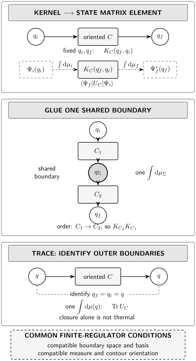
Boundary operations at a common finite regulator. Fixed $q_i,q_f$ define $K_C(q_f,q_i)$ with no endpoint integration. Attaching $\Psi_i$ and $\Psi_f^*$ adds one integration over each outer endpoint. Gluing $C_1$ to $C_2$ inserts one compatible resolution of the identity and therefore one $\mathrm d\mu_\Sigma(q_\Sigma)$; the two induced interface orientations are opposite. A trace identifies $q_f=q_i=q$ and integrates that diagonal once. Contour arrows show operator order, so the glued integrand is $K_{C_2}K_{C_1}$. The schematic is not to scale.

The Euclidean oscillator checks both gluing and projection

For a unit-mass harmonic oscillator of frequency $\omega>0$, the exact Euclidean kernel for $T>0$ is

$$\begin{gathered} K_E(q_f,T;q_i,0) = \left( \frac{\omega}{2\pi\sinh\omega T} \right)^{1/2} \\ {}\times \exp\!\left[ -\frac{\omega}{2\sinh\omega T} \Xi_T(q_f,q_i) \right], \\ \Xi_T(q_f,q_i) = (q_f^2+q_i^2)\cosh\omega T \\ {}\quad -2q_fq_i. \end{gathered}$$

It obeys the semigroup law

$$\begin{gathered} \int_{-\infty}^{\infty}\mathrm dq\, K_E(q_f,T_2;q,0) \\ {}\times K_E(q,T_1;q_i,0) \\ {}= K_E(q_f,T_1+T_2;q_i,0). \end{gathered}$$

This is a direct Gaussian check of the abstract identity insertion. Combining the two quadratic exponents and using

$$\coth a+\coth b = \frac{\sinh(a+b)}{\sinh a\,\sinh b}$$

reproduces both the exponent and the normalization at $T_1+T_2$. A missing seam integration, a second seam integration, or an inconsistent measure fails this test.

For large $T$,

$$\begin{gathered} K_E(q_f,T;q_i,0) = e^{-\omega T/2} \left(\frac{\omega}{\pi}\right)^{1/2} \\ {}\times \exp\!\left[-\frac{\omega}{2}(q_f^2+q_i^2)\right] \\ {}\times \left[1+O(e^{-\omega T})\right] \\ {}= e^{-E_0T}\, \psi_0(q_f)\psi_0(q_i) \\ {}\quad +O(e^{-E_1T}), \end{gathered}$$

where

$$E_0=\frac{\omega}{2}, \qquad \psi_0(q)= \left(\frac{\omega}{\pi}\right)^{1/4} e^{-\omega q^2/2}.$$

The same kernel therefore validates composition at finite $T$ and displays ground-state factorization as $T\to\infty$.

Euclidean evolution selects the lowest overlapping state

The general statement is spectral. Let $H$ be self-adjoint and bounded below, and, for clarity, suppose the regulated problem has a discrete orthonormal spectrum. For

$$|\chi\rangle=\sum_n c_n|n\rangle, \qquad H|n\rangle=E_n|n\rangle,$$

Euclidean evolution gives

$$\begin{aligned} e^{-TH}|\chi\rangle &= c_0e^{-E_0T}|0\rangle \\ &\quad+ \sum_{n>0}c_n e^{-E_nT}|n\rangle. \end{aligned}$$

If the ground state is unique, $c_0\ne0$, and $\Delta=E_1-E_0>0$, then after normalization

$$\frac{e^{-TH}|\chi\rangle} {\|e^{-TH}|\chi\rangle\|} = \frac{c_0}{|c_0|}|0\rangle +O(e^{-T\Delta}).$$

The phase $c_0/|c_0|$ has no physical effect. Under the same hypotheses, and for an operator whose relevant matrix elements are controlled,

$$\lim_{T\to\infty} \frac{ \langle\chi|e^{-TH}\widehat Oe^{-TH}|\chi\rangle }{ \langle\chi|e^{-2TH}|\chi\rangle } = \langle0|\widehat O|0\rangle.$$

Each hypothesis matters:

• If $c_0=0$, the limit selects the lowest-energy state having nonzero overlap with $|\chi\rangle$, not the ground state.
• If the ground space is degenerate, the limit retains the projection of $|\chi\rangle$ into that space; Euclidean evolution alone does not choose a unique vector.
• Without a positive gap, convergence need not be exponentially fast.
• Taking $T\to\infty$ at a fixed regulator is not the same operation as removing the ultraviolet regulator, taking infinite volume, or sending a mass to zero.

The large-Euclidean-time argument and its relation to energy gaps and correlation decay are given in Zinn-Justin 2021, §§ 2.4–2.5.1, pp. 25–28.

A Euclidean half-space prepares the regulated free-scalar vacuum

Now retain finitely many real normal-mode coordinates of a free scalar. Their Euclidean action on the half-line $\tau\le 0$ is

$$\begin{aligned} S_E[q] &= \frac12 \int_{-\infty}^{0}\mathrm d\tau \\ &\quad\times \left( \dot q^{\mathsf T}\dot q +q^{\mathsf T}\Omega_\Lambda^2q \right), \\ \Omega_\Lambda &= \Omega_\Lambda^{\mathsf T}>0. \end{aligned}$$

To prepare a wave function of the boundary value $\varphi$, impose

$$\begin{aligned} q(0)&=\varphi, \\ q(\tau)&\longrightarrow0 \quad(\tau\longrightarrow-\infty). \end{aligned}$$

The unique classical solution is

$$q_{\mathrm{cl}}(\tau) = e^{\Omega_\Lambda\tau}\varphi.$$

Because $\dot q_{\mathrm{cl}}=\Omega_\Lambda q_{\mathrm{cl}}$,

$$\begin{aligned} S_E[q_{\mathrm{cl}}] &= \int_{-\infty}^{0}\mathrm d\tau\, \varphi^{\mathsf T} e^{\Omega_\Lambda\tau} \Omega_\Lambda^2 e^{\Omega_\Lambda\tau} \varphi \\ &= \frac12\, \varphi^{\mathsf T}\Omega_\Lambda\varphi. \end{aligned}$$

Write $q=q_{\mathrm{cl}}+\eta$ with $\eta(0)=\eta(-\infty)=0$. The cross term vanishes by the classical equation and the endpoint conditions, while the fluctuation integral over $\eta$ is independent of $\varphi$. Consequently the half-space functional integral prepares

$$\begin{aligned} \Psi_{0,\Lambda}(\varphi) &= \mathcal N_\Lambda \exp\!\left( -\frac12\varphi^{\mathsf T} \Omega_\Lambda\varphi \right), \\ \mathcal N_\Lambda &= \left( \frac{\det\Omega_\Lambda}{\pi^M} \right)^{1/4}, \end{aligned}$$

after normalizing in $\mathrm d^M\varphi$. This is the same regulated Gaussian found canonically on the Schrödinger Wave Functionals page, now obtained by Euclidean preparation rather than by solving the functional Schrödinger equation.

Strict positivity of $\Omega_\Lambda$ is essential. A zero-frequency mode has no decaying half-line solution for a generic boundary value, and the formal Gaussian is constant along that direction and therefore nonnormalizable. Such modes require a separate infrared treatment.

Contour orientation records preparation and evolution

A Lorentzian segment implements $e^{-iH\Delta t}$, while a downward Euclidean segment implements $e^{-H\Delta\tau}$. Attaching a long Euclidean segment before Lorentzian evolution is therefore a state-preparation operation. Its orientation determines which end is initial and which is final, and the final wave function enters as a bra, hence as $\Psi_f^*$.

This elementary contour grammar should not be confused with a complete pole prescription. In real-time vacuum amplitudes, boundary wave functions and their asymptotic damping can induce the Feynman boundary value, as shown explicitly for the free scalar in Schwartz 2014, § 14.4.1, pp. 265–266. General contour deformation, the $i0$ prescription, and doubled real-time contours require additional assumptions and are developed on their own pages.

Where the finite construction stops

The formulas above concern temporal state boundaries in a regulated scalar theory. They do not by themselves determine spatial boundary conditions, self-adjoint extensions, gauge-edge degrees of freedom, or constraint measures. Those problems can change the boundary configuration space and the very identity used for gluing.

Nor does the finite construction establish a continuum sewing measure. Before removing a regulator, one must control normalization, counterterms, possible boundary counterterms, zero modes, and the compatibility of the two sides of an interface. Interacting vacuum preparation can also require phase information and limiting prescriptions beyond the positive Euclidean Gaussian example.

Common pitfalls

Treating fixed boundary data as a prepared state. A fixed value $q_i$ labels a generalized configuration eigenstate and defines a kernel. A normalizable state requires a wave function or a separate preparation condition, followed by the appropriate endpoint integration.

Integrating a seam twice. Gluing inserts one resolution of the identity, so there is exactly one integral over the shared configuration. The two kernels each depend on that same variable; neither supplies a second measure.

Claiming that long Euclidean time always gives a unique vacuum. The initial boundary data must overlap the ground space. Uniqueness and exponential convergence additionally require a nondegenerate ground state and a positive gap at the regulator under discussion.

Calling every trace thermal. The identity $\operatorname{Tr}U=\int\mathrm d\mu(q)K(q,q)$ is structural. A thermal interpretation requires $U=e^{-\beta H}$, a specified Hilbert space, and normalization by the partition function.

Check your understanding

1. Count the endpoint integrations

Starting from $K_C(q_f,q_i)$, write the expressions for (a) a matrix element between two wave functions, (b) a composition across one seam, and (c) a trace. State which variables are integrated in each case.

Solution

For a matrix element, integrate $q_i$ and $q_f$ against $\Psi_i(q_i)$ and $\Psi_f^*(q_f)$. For a composition, keep the outer endpoints fixed and integrate the single shared variable $q_\Sigma$ once. For a trace, set $q_f=q_i=q$ and integrate that diagonal variable once.

2. Extract the oscillator ground state

Use $\sinh\omega T\sim e^{\omega T}/2$ and $\cosh\omega T\sim e^{\omega T}/2$ to find the leading large-$T$ form of the Euclidean oscillator kernel.

Solution

The prefactor becomes $e^{-\omega T/2}(\omega/\pi)^{1/2}$, while the exponent becomes $-\omega(q_f^2+q_i^2)/2+O(e^{-\omega T})$. Thus

$$\begin{aligned} K_E(q_f,T;q_i,0) &\sim e^{-\omega T/2} \\ &\quad\times \psi_0(q_f)\psi_0(q_i), \end{aligned}$$

with $\psi_0(q)=(\omega/\pi)^{1/4}e^{-\omega q^2/2}$.

3. Diagnose failed vacuum selection

Suppose $c_0=0$, but $c_k\ne0$ and $E_k$ is the lowest energy with nonzero overlap. What state does normalized Euclidean evolution approach?

Solution

Factor out $e^{-E_kT}$ rather than $e^{-E_0T}$. The normalized state approaches $(c_k/|c_k|)|k\rangle$ if that level is nondegenerate and separated from the next overlapping level. If it is degenerate, the surviving state is the normalized projection of $|\chi\rangle$ into that eigenspace.

4. Check the half-space boundary action

For one mode, substitute $q_{\mathrm{cl}}(\tau)=\varphi e^{\omega\tau}$ into the Euclidean action and evaluate it.

Solution

Since $\dot q_{\mathrm{cl}}=\omega q_{\mathrm{cl}}$,

$$\begin{aligned} S_E[q_{\mathrm{cl}}] &= \frac12\int_{-\infty}^{0}\mathrm d\tau\, 2\omega^2\varphi^2e^{2\omega\tau} \\ &= \frac12\omega\varphi^2. \end{aligned}$$

The boundary dependence of the path integral is therefore $e^{-\omega\varphi^2/2}$.

Where to continue

• Canonical–Functional Crosswalk for Regulated Systems compares kernels, states, operators, and correlators across the two formulations.
• Lorentzian Boundary Conditions and the $i\varepsilon$ Prescription develops the asymptotic condition behind real-time vacuum amplitudes.
• Closed-Time-Path Grammar treats doubled forward and backward real-time branches.
• Thermal Density Operators and the KMS Condition supplies the extra structure that turns Euclidean trace closure into a thermal state.

References

• Schwartz, Matthew D. Quantum Field Theory and the Standard Model. Cambridge University Press, 2014. doi:10.1017/9781139540940.
• Weinberg, Steven. The Quantum Theory of Fields. Volume I: Foundations. Cambridge University Press, 1995. doi:10.1017/CBO9781139644167.
• Zinn-Justin, Jean. Quantum Field Theory and Critical Phenomena. 5th ed., Oxford University Press, 2021. doi:10.1093/oso/9780198834625.001.0001.