Thermal Density Operators and the KMS Condition

The Kubo–Martin–Schwinger condition recognizes thermal equilibrium from the complex-time behavior of correlation functions. In a finite system it follows from one exact fact—cyclicity of the Gibbs trace. In an infinite system the same analytic boundary relation remains meaningful even when no global density matrix exists. This extra structure is essential: a state can be stationary without being thermal at any single temperature.

The analytic strip appears in Kubo 1957, § 4, p. 579, Eq. (4.13) and the following analyticity paragraph through Eqs. (4.14)–(4.15), while Martin and Schwinger 1959, § V, pp. 1357–1359, especially Eqs. (5.11)–(5.18) derive the thermal boundary conditions and the bosonic or fermionic mode families.

Required background. Hilbert Positivity and Unitary Evolution fixes states and adjoints. Retarded, Advanced, and Spectral Correlators fixes causal correlators and the site Fourier transform. Helpful background. Thermal OPE and KMS Crossing develops the conformal specialization.

The positive KMS strip

Set $k_{\mathrm B}=\hbar=1$, fix $\beta>0$, and let

$$\rho_\beta=\frac{e^{-\beta H}}{Z_\beta}, \qquad Z_\beta=\operatorname{Tr}e^{-\beta H}, \qquad A(t)=e^{iHt}Ae^{-iHt}.$$

The trace derivation below is rigorous as written in finite dimension. In an infinite-dimensional trace-class realization, take $e^{-\beta H}$ to be trace class and restrict first to bounded entire analytic elements of the $H$-dynamics, with every reordered product below trace class, so that trace cyclicity applies. Unbounded fields require a separate domain analysis and are not covered merely by writing a formal trace. These are mathematical hypotheses, not cosmetic qualifications.

There are two equivalent strip conventions; mixing them reverses the ordering. This page uses the positive strip

$$0<\operatorname{Im}z<\beta$$

and assigns to it the function

$$F_{B,A}(z)=\langle B A(z)\rangle_\beta.$$

Its lower and upper boundary values are

$$F_{B,A}(t)=\langle B A(t)\rangle_\beta, \qquad F_{B,A}(t+i\beta)=\langle A(t)B\rangle_\beta.$$

Thus the same analytic function reaches the two operator orderings on opposite sides of the strip. Equivalently,

$$\boxed{ \langle A(t)B\rangle_\beta =\langle B A(t+i\beta)\rangle_\beta }.$$

If instead one defines $G_{A,B}(z)=\langle A(z)B\rangle_\beta$, its natural strip is the negative one, $-\beta<\operatorname{Im}z<0$, and

$$G_{A,B}(t-i\beta)=\langle B A(t)\rangle_\beta.$$

Both versions express the same condition. A reliable calculation writes the operator order on both boundaries before choosing the sign of the strip.

Trace cyclicity gives the boundary exchange

The imaginary shift follows directly from the Heisenberg convention:

$$e^{-\beta H}A(t)e^{\beta H}=A(t+i\beta), \qquad e^{-\beta H}A(t)=A(t+i\beta)e^{-\beta H}.$$

Now move the factors without skipping a step:

$$\begin{aligned} \langle A(t)B\rangle_\beta &=\frac1{Z_\beta}\operatorname{Tr} \!\left(e^{-\beta H}A(t)B\right)\\ &=\frac1{Z_\beta}\operatorname{Tr} \!\left(B e^{-\beta H}A(t)\right)\\ &=\frac1{Z_\beta}\operatorname{Tr} \!\left(B A(t+i\beta)e^{-\beta H}\right)\\ &=\langle B A(t+i\beta)\rangle_\beta. \end{aligned}$$

In a finite-dimensional system this also supplies the analytic continuation explicitly. In an infinite-dimensional trace-class setting, analyticity and boundary continuity require the corresponding domain and growth control. Merely checking the equality at two formal endpoints is not the full KMS property.

The converse is useful in the finite type-I setting. Suppose $H|n\rangle=E_n|n\rangle$ and a faithful stationary state has weights $p_n$. Applying KMS to matrix units that connect levels $m$ and $n$ forces

$$\frac{p_n}{p_m}=e^{-\beta(E_n-E_m)}.$$

If the full matrix algebra is tested, these ratios reconstruct the single normalized state $p_n\propto e^{-\beta E_n}$, including equal weights within degenerate eigenspaces. Sector-dependent normalizations can remain only for a smaller direct-sum observable algebra with central superselection blocks that no observable connects. KMS is therefore not a test of one favored correlator; it is an all-observable equilibrium condition.

Intrinsic equilibrium without a density matrix

In an infinite system, $e^{-\beta H}$ is generally not trace class in the representation of interest. The trace calculation motivates the definition but cannot be used as the definition. Let $\mathfrak A$ be a $C^*$-algebra of bounded observables, $\alpha_t$ a strongly continuous time-evolution automorphism, and $\omega$ a positive normalized state. The positive-strip formulation requires, for every $X,Y\in\mathfrak A$, a function continuous and bounded on the closed strip, analytic inside it, and satisfying

$$F_{X,Y}(t)=\omega\!\left(X\alpha_t(Y)\right), \qquad F_{X,Y}(t+i\beta)=\omega\!\left(\alpha_t(Y)X\right).$$

The algebra, dynamics, inverse temperature, analytic domain, and observable class are all part of the claim. On a norm-dense algebra of entire analytic elements the boundary identity has an equivalent algebraic form; continuity then extends it. C*-Dynamical Systems and the KMS Condition develops that theorem-level formulation. The original passage from local Gibbs descriptions to intrinsic equilibrium is treated in Haag, Hugenholtz, and Winnink 1967, §§ 1–3, pp. 215–229.

Finite Gibbs modular flow

For a faithful finite-dimensional Gibbs state, modular flow packages the same imaginary-time relation in operator form. If

$$\begin{gathered} K=K^\dagger, \qquad \Xi=\operatorname{Tr}e^{-\beta K},\\ \rho=\frac{e^{-\beta K}}{\Xi}, \qquad \alpha_t^K(A)=e^{iKt}Ae^{-iKt}. \end{gathered}$$

then its modular Hamiltonian is

$$K_{\mathrm{mod}}=-\log\rho =\beta K+\log\Xi,$$

and the dimensionless modular parameter $s$ acts by

$$\sigma_s^\rho(A)=\rho^{is}A\rho^{-is} =\alpha_{-\beta s}^K(A).$$

On the finite-dimensional Hilbert–Schmidt operator space, the modular operator acts as

$$\Delta_\rho(X)=\rho X\rho^{-1} =e^{-\beta\mathcal L_K}X, \qquad \mathcal L_K(X)=KX-XK.$$

Thus the $K$-generated evolution parameter and modular time are related by $t=-\beta s$ with the conventions used here; $K$ and $K_{\mathrm{mod}}$ are not the same generator. In the infinite-dimensional theory $\Delta_\rho$ is generally an unbounded positive operator on a natural dense domain, so the displayed formula is not an everywhere-defined matrix identity. Modular Automorphisms, Conjugations, and Standard Forms develops the Hilbert–Schmidt realization, while Modular Dynamics and Equilibrium Representations owns the general representation-theoretic statement and domain hypotheses.

Stationarity is not thermality

Every KMS state is stationary under the declared dynamics. The converse fails. For example, take an equally spaced three-level Hamiltonian and a faithful diagonal state,

$$H=\operatorname{diag}(0,\Delta,2\Delta), \qquad \rho=\operatorname{diag}\!\left(\frac12,\frac13,\frac16\right).$$

Here $\Delta>0$. Because $[\rho,H]=0$, the state is stationary. KMS on the $0\leftrightarrow1$ transition would require $e^{-\beta\Delta}=2/3$, whereas the $1\leftrightarrow2$ transition requires $e^{-\beta\Delta}=1/2$. No single $\beta$ satisfies both. This is why a three-level example is more revealing than a faithful two-level state: one noninverted population ratio can define an effective positive $\beta$, but several transitions test whether one common temperature organizes the full algebra. A population inversion lies outside the positive-temperature convention of this page and requires a separately declared negative-temperature or reversed-dynamics treatment.

Infinite-Volume KMS States, Passivity, and Phase Multiplicity explains how local limits can yield more than one extremal KMS state at the same temperature. KMS does not assert that a thermodynamic limit exists, is unique, or is represented by a global Gibbs operator.

Grand-canonical time and chemical twists

For commuting conserved charges, define

$$K=H-\sum_a\mu_aQ_a, \qquad \rho_{\beta,\mu}=\frac{e^{-\beta K}}{\Xi}, \qquad [H,Q_a]=[Q_a,Q_b]=0.$$

With $K$-generated evolution, the KMS equation has exactly the form already derived, with $H$ replaced by $K$. Physical response is often labeled by $H$-generated time instead. For one charge, adopt the field convention

$$[Q,A]=-q_A A.$$

Then $e^{\beta\mu Q}A e^{-\beta\mu Q}=e^{-\beta\mu q_A}A$, and the $H$-time boundary relation becomes

$$\langle A_H(t)B\rangle_{\beta,\mu} =e^{-\beta\mu q_A} \langle B A_H(t+i\beta)\rangle_{\beta,\mu}.$$

The sign is fixed by the displayed commutator. If a source defines charge with the opposite sign, the twist changes accordingly. Conserved Charges and Grand-Canonical States treats stability, charge sectors, and which generator labels a spectrum; Imaginary Time and Matsubara Frequencies translates the same twist into a Euclidean derivative or shifted frequency.

Statistics, time ordering, and detailed balance

Ordinary trace cyclicity inserts no fermionic sign. The minus sign appears when odd operators are exchanged by imaginary-time ordering. It is clearest to define bosonic and fermionic Green functions separately. For $0<\tau<\beta$,

$$G_B(\tau)=\langle \mathrm T_\tau\phi(\tau)\phi^\dagger(0)\rangle_\beta, \qquad G_F(\tau)=-\langle \mathrm T_\tau\psi(\tau)\psi^\dagger(0)\rangle_\beta.$$

Wrapping an insertion around the trace gives

$$G_B(\tau+\beta)=G_B(\tau), \qquad G_F(\tau+\beta)=-G_F(\tau).$$

Consequently bosons use $\omega_n=2\pi nT$ and fermions use $\omega_n=(2n+1)\pi T$. A $(-1)^F$ insertion changes the closure of an odd field and defines a supertrace or index-like object; it does not turn graded cyclicity into an ordinary thermal trace. Thermal Boundary Conditions and Graded Traces develops that distinction.

KMS also becomes a frequency-domain detailed-balance identity. Declare

$$G^>_{AB}(t)=\langle A(t)B\rangle_\beta, \qquad G^<_{AB}(t)=\langle B A(t)\rangle_\beta,$$

and use the site transform $G(\omega)=\int_{-\infty}^{\infty}\mathrm dt\,e^{+i\omega t}G(t)$. Shifting the contour through the analytic strip gives

$$G^>_{AB}(\omega)=e^{\beta\omega}G^<_{AB}(\omega),$$

provided the boundary values and falloff justify the shift. With the grand-canonical convention $[Q,A]=-q_AA$ above and $H$-generated time, the same calculation instead gives

$$G^>_{AB}(\omega) =e^{\beta(\omega-\mu q_A)}G^<_{AB}(\omega)$$

for a charge-balanced pair. Alternate Fourier phases or a different time generator change the visible exponential, so the convention must accompany the formula. Thermal Propagators and Spectral Representations turns this relation into thermal occupation factors, and KMS Relations and Fluctuation–Dissipation adds the response-function dictionary.

Harmonic-oscillator boundary check

For

$$H=\omega\!\left(a^\dagger a+\frac12\right), \qquad a(t)=e^{-i\omega t}a, \qquad n_B(\omega)=\frac1{e^{\beta\omega}-1},$$

the positive-strip function for $A=a$ and $B=a^\dagger$ is

$$F_{a^\dagger,a}(z) =\langle a^\dagger a(z)\rangle_\beta =n_B e^{-i\omega z}.$$

Its two boundaries are

$$\begin{aligned} F_{a^\dagger,a}(t) &=n_Be^{-i\omega t} =\langle a^\dagger a(t)\rangle_\beta,\\ F_{a^\dagger,a}(t+i\beta) &=n_Be^{\beta\omega}e^{-i\omega t} =(1+n_B)e^{-i\omega t} =\langle a(t)a^\dagger\rangle_\beta. \end{aligned}$$

This one ladder-operator calculation checks the strip direction, the order exchanged at the upper boundary, and the Bose factor, but by itself it fixes only a relation involving the mean occupation. For an arbitrary stationary diagonal oscillator state, testing every bounded adjacent matrix-unit pair $|n+1\rangle\langle n|$ and $|n\rangle\langle n+1|$ demands $p_{n+1}/p_n=e^{-\beta\omega}$ level by level. A nongeometric distribution therefore fails KMS even though it commutes with $H$.

Equilibrium tests and their logical strength

• Stationarity preserves expectations under real-time translation. It does not determine imaginary-time analyticity or one common temperature.
• KMS equilibrium imposes the strip and boundary relation for every bounded observable pair in the declared $C^*$-algebra relative to a declared dynamics.
• Detailed balance is a frequency or transition-rate symmetry whose exact expression depends on the correlator, generator, grading, and Fourier convention.
• Passivity forbids net work extraction by every admissible cyclic operation on one copy, in the sense of Pusz and Woronowicz 1978, Definition 1.1 and Theorem 1.1, pp. 276–277. It is stronger than stationarity but does not by itself force a KMS state.
• Complete passivity requires every finite tensor power of the state to be passive. In the same $C^*$-dynamical setting, the completely passive states are precisely KMS states at nonnegative inverse temperature or ground states Pusz and Woronowicz 1978, § 1, p. 278, Definition 1.3, Theorem 1.4, and the following remark.

Retaining the ground-state alternative and the allowed-operation hypotheses prevents the passivity theorem from being overstated. The shared equilibrium convention table keeps finite definitions, limiting constructions, and inference ceilings separate.

The figure makes the two complex-time boundaries and the later conditional branches visible at once. Inspect where operator order changes, then follow how a Euclidean representation, field parity, conserved insertion, and Fourier convention jointly fix the closure and mode lattice around the circle.

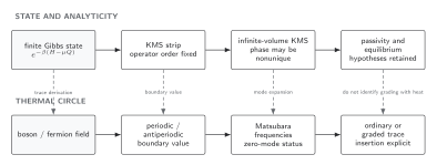
The upper panel fixes the positive-strip convention: $F_{B,A}(t)=\omega(B A(t))$ on the lower edge and $F_{B,A}(t+i\beta)=\omega(A(t)B)$ on the upper edge. A finite Gibbs trace proves this relation by cyclicity; the same strip condition defines equilibrium without a global trace, while constructing a thermodynamic-limit state is separate and phases may be nonunique. The lower panel shows how an ordinary thermal trace yields bosonic or fermionic Matsubara families and how a $(-1)^F$ insertion changes fermion closure rather than defining heat. Complete passivity selects a KMS or ground state under the stated hypotheses. The diagram is schematic and not to scale.

Exercises

1. Let $H|n\rangle=E_n|n\rangle$ and $R_{nm}=|n\rangle\langle m|$. For $E_n>E_m$, evaluate the two KMS boundaries for $A=R_{nm}$ and $B=R_{mn}$ in a diagonal state $\rho=\sum_kp_k|k\rangle\langle k|$. Show that KMS requires $p_n/p_m=e^{-\beta(E_n-E_m)}$.

Solution

Write $\Delta=E_n-E_m>0$. Since $R_{nm}(t)=e^{i\Delta t}R_{nm}$,

$$\langle R_{nm}(t)R_{mn}\rangle =p_n e^{i\Delta t}.$$

The other boundary is

$$\langle R_{mn}R_{nm}(t+i\beta)\rangle =p_m e^{i\Delta t}e^{-\beta\Delta}.$$

Equality gives $p_n=p_m e^{-\beta\Delta}$. Testing all matrix units makes the condition sufficient for the Gibbs weights on every connected sector.

2. Let $K|n\rangle=\kappa_n|n\rangle$ in finite dimension and $\rho=e^{-\beta K}/\Xi$. For $R_{mn}=|m\rangle\langle n|$, compute $\sigma_s^\rho(R_{mn})$ and $\Delta_\rho(R_{mn})$. Verify both the rescaling $\sigma_s^\rho=\alpha_{-\beta s}^K$ and the relation $\Delta_\rho=e^{-\beta\mathcal L_K}$.

Solution

The Gibbs eigenvalues are $p_n=e^{-\beta\kappa_n}/\Xi$, so

$$\rho^{is}R_{mn}\rho^{-is} =\left(\frac{p_m}{p_n}\right)^{is}R_{mn} =e^{-i\beta s(\kappa_m-\kappa_n)}R_{mn}.$$

But $\alpha_t^K(R_{mn})=e^{it(\kappa_m-\kappa_n)}R_{mn}$, hence the first expression equals $\alpha_{-\beta s}^K(R_{mn})$. Similarly,

$$\Delta_\rho(R_{mn}) =\frac{p_m}{p_n}R_{mn} =e^{-\beta(\kappa_m-\kappa_n)}R_{mn}.$$

Since $\mathcal L_K(R_{mn})=(\kappa_m-\kappa_n)R_{mn}$, this is exactly $e^{-\beta\mathcal L_K}R_{mn}$. Matrix units span the finite-dimensional Hilbert–Schmidt space, so the relations hold on the whole space.

3. Starting from $G^>(t)=G^<(t+i\beta)$ and the transform $G(\omega)=\int\mathrm dt\,e^{i\omega t}G(t)$, derive detailed balance. State the analytic step that could fail.

Solution

Set $u=t+i\beta$, so $t=u-i\beta$ and $e^{i\omega t}=e^{\beta\omega}e^{i\omega u}$. The integration line is initially $\operatorname{Im}u=\beta$. If analyticity and falloff permit moving it to the real axis without crossing singularities or retaining end segments, then

$$G^>(\omega)=e^{\beta\omega}G^<(\omega).$$

The contour deformation—not a formal substitution of complex time—is the decisive step.

4. Let $[a,a^\dagger]=1$, $[Q,a]=-qa$, and $K=H-\mu Q$ for a charged bosonic oscillator with $[H,a]=-\omega a$. Use $H$-generated time to show that KMS gives the occupation number $n=[e^{\beta(\omega-\mu q)}-1]^{-1}$.

Solution

The $H$-time twisted relation is

$$\langle a(t)a^\dagger\rangle =e^{-\beta\mu q} \langle a^\dagger a(t+i\beta)\rangle.$$

Using $a(t)=e^{-i\omega t}a$ and $aa^\dagger=1+a^\dagger a$, the left side is $(1+n)e^{-i\omega t}$ and the right side is $e^{-\beta\mu q}n e^{-i\omega t}e^{\beta\omega}$. Therefore $1+n=n e^{\beta(\omega-\mu q)}$, which gives the stated Bose occupation. For $\beta>0$, normalizability requires $\omega-\mu q>0$. Equality produces the bosonic zero-mode divergence, while $\omega-\mu q<0$ makes $e^{-\beta K}$ non-normalizable.

References

• Haag, Rudolf, Nico M. Hugenholtz, and Marius Winnink. “On the Equilibrium States in Quantum Statistical Mechanics.” Communications in Mathematical Physics 5 (1967): 215–236. doi:10.1007/BF01646342.
• Kubo, Ryogo. “Statistical-Mechanical Theory of Irreversible Processes. I. General Theory and Simple Applications to Magnetic and Conduction Problems.” Journal of the Physical Society of Japan 12, no. 6 (1957): 570–586. doi:10.1143/JPSJ.12.570.
• Martin, Paul C., and Julian Schwinger. “Theory of Many-Particle Systems. I.” Physical Review 115, no. 6 (1959): 1342–1373. doi:10.1103/PhysRev.115.1342.
• Pusz, Wiesław, and Stanisław L. Woronowicz. “Passive States and KMS States for General Quantum Systems.” Communications in Mathematical Physics 58, no. 3 (1978): 273–290. doi:10.1007/BF01614224.