Thermal OPE and KMS Crossing

The thermal bootstrap combines two exact statements about a local correlator: the OPE converges when the insertions fit inside a contractible ball, and cyclicity of the normalized thermal trace relates different Euclidean orderings. Their overlap gives a crossing equation for products of vacuum OPE coefficients and thermal one-point coefficients. This is KMS consistency, not a torus modular transformation.

Required background. Thermal states and one-point data fixes the ensemble and one-point normalization, while OPE convergence and associativity fixes the local expansion. Helpful background. Lorentzian boundary prescriptions explains how distinct real-time orderings arise from different analytic continuations.

Local OPE data in a periodic Euclidean geometry

Consider an identical bosonic scalar primary $\phi$ of dimension $\Delta_\phi$ on

$$S^1_\beta\times\mathbb R^{d-1}$$

in the neutral canonical state. Define the normalized, Euclidean-time-ordered correlator

$$G_\beta(\tau,\mathbf x) =\left\langle \phi(\tau,\mathbf x)\phi(0,\mathbf0) \right\rangle_\beta, \qquad 0<\tau<\beta.$$

Let

$$r=\sqrt{\tau^2+\lvert\mathbf x\rvert^2}, \qquad \eta=\frac{\tau}{r}, \qquad \nu=\frac{d-2}{2}.$$

The two insertions can be enclosed in a flat ball that does not wrap the thermal circle when

$$r<\beta.$$

In that domain, insert the vacuum OPE and take thermal one-point functions. For symmetric traceless primaries of even spin $J$,

$$G_\beta(\tau,\mathbf x) =\sum_{\mathcal O\in\phi\times\phi} \frac{a_{\mathcal O}}{\beta^{\Delta_{\mathcal O}}} C_J^{(\nu)}(\eta) r^{\Delta_{\mathcal O}-2\Delta_\phi},$$

where

$$a_{\mathcal O} =\frac{f_{\phi\phi\mathcal O}b_{\mathcal O}} {c_{\mathcal O}} \frac{J!}{2^J(\nu)_J}.$$

Here $c_{\mathcal O}$ normalizes the vacuum two-point function, $f_{\phi\phi\mathcal O}$ is the vacuum three-point coefficient, and $b_{\mathcal O}$ is the thermal one-point coefficient. The identity has $a_{\mathbf1}=1$. This convention and convergence domain follow Iliesiu et al. 2018, § 2.1, eqs. (2.5)–(2.12).

The formula is written for $d>2$, where Gegenbauer polynomials are a convenient basis. In $d=2$, take the appropriate $\nu\to0$ limit and use the two angular harmonics rather than substituting $\nu=0$ into the normalization blindly.

Unlike an identical-scalar vacuum four-point decomposition, the coefficients $a_{\mathcal O}$ are not generally nonnegative. Even when $c_{\mathcal O}>0$, the product $f_{\phi\phi\mathcal O}b_{\mathcal O}$ can have either sign. Thermal crossing is therefore a linear consistency equation without the default scalar positivity cone of the ordinary unitary bootstrap.

KMS from cyclicity and ordering

For operators $A,B$ and $0<\tau<\beta$,

$$\begin{aligned} \langle A(\tau)B(0)\rangle_\beta &=\frac1Z \operatorname{Tr} \left(e^{-(\beta-\tau)H}A(0)e^{-\tau H}B(0)\right)\\ &=\frac1Z \operatorname{Tr} \left(e^{-\tau H}B(0)e^{-(\beta-\tau)H}A(0)\right)\\ &=\langle B(\beta-\tau)A(0)\rangle_\beta. \end{aligned}$$

For an identical scalar, spatial rotations give

$$G_\beta(\tau,\mathbf x) =G_\beta(\beta-\tau,-\mathbf x) =G_\beta(\beta-\tau,\mathbf x).$$

This reflection around $\tau=\beta/2$ is the scalar KMS crossing equation Iliesiu et al. 2018, § 2.2, eqs. (2.25)–(2.29).

For fermionic Euclidean-time-ordered correlators, moving an odd operator through the thermal trace introduces the graded KMS sign. A chemical potential replaces ordinary periodicity by a charge-dependent twist. For nonidentical operators, KMS reverses their order. These distinctions must be fixed before analytic continuation: a Wightman, time-ordered, retarded, and Euclidean correlator are different boundary values of analytic functions, not interchangeable notations.

The explicit thermal crossing equation

Define the KMS image point

$$r'=\sqrt{(\beta-\tau)^2+\lvert\mathbf x\rvert^2}, \qquad \eta'=\frac{\beta-\tau}{r'}.$$

Where both $r<\beta$ and $r'<\beta$, the same OPE data can be used on the two sides:

$$\sum_{\mathcal O} a_{\mathcal O}\beta^{-\Delta_{\mathcal O}} C_J^{(\nu)}(\eta) r^{\Delta_{\mathcal O}-2\Delta_\phi} = \sum_{\mathcal O} a_{\mathcal O}\beta^{-\Delta_{\mathcal O}} C_J^{(\nu)}(\eta') {r'}^{\Delta_{\mathcal O}-2\Delta_\phi}.$$

At $\tau=\beta/2$, the correlator is even in

$$t=\tau-\frac\beta2.$$

Therefore every odd derivative obeys

$$\left. \partial_\tau^{2n+1} G_\beta(\tau,\mathbf x) \right|_{\tau=\beta/2}=0,$$

provided the derivative and OPE sum may be interchanged. Inserting the block expansion produces linear sum rules for $a_{\mathcal O}$. A truncated sum rule needs a bound on the differentiated OPE tail; convergence of the undifferentiated series alone is not enough near the boundary $r=\beta$.

The unknowns are the products $f_{\phi\phi\mathcal O}b_{\mathcal O}/c_{\mathcal O}$. If the vacuum spectrum and OPE coefficients are known independently, the equations constrain $b_{\mathcal O}$. Otherwise a single thermal two-point function determines only those products and only for operators appearing in $\phi\times\phi$.

A generalized-free benchmark with a tail bound

Normalize the zero-temperature two-point function to

$$\langle\phi(x)\phi(0)\rangle =\frac1{\lvert x\rvert^{2\Delta_\phi}}.$$

The bosonic generalized-free thermal image sum is

$$G_\beta^{\mathrm{GFF}}(\tau,\mathbf x) =\sum_{m\in\mathbb Z} \frac1{ \left[(\tau+m\beta)^2 +\lvert\mathbf x\rvert^2\right]^{\Delta_\phi}}.$$

It is absolutely convergent for $\Delta_\phi>1/2$. Relabeling $m\mapsto-m-1$ gives

$$G_\beta^{\mathrm{GFF}}(\beta-\tau,\mathbf x) =G_\beta^{\mathrm{GFF}}(\tau,\mathbf x),$$

so KMS is exact. Expanding the nonzero images near the origin reproduces the mean-field thermal one-point coefficients; thermal inversion gives the same data Iliesiu et al. 2018, § 4, eqs. (4.2)–(4.8).

Now truncate to $\lvert m\rvert\le M$. Let $u=\lvert\tau\rvert/\beta$ and assume $M>u$. Since each omitted image has distance at least $(m-u)\beta$, the remainder satisfies

$$\begin{aligned} \lvert R_M\rvert &\le2\beta^{-2\Delta_\phi} \sum_{m=M+1}^{\infty}(m-u)^{-2\Delta_\phi}\\ &\le \frac{2\beta^{-2\Delta_\phi}} {2\Delta_\phi-1} (M-u)^{1-2\Delta_\phi}. \end{aligned}$$

This controls the correlator tail uniformly in $\mathbf x$ because nonzero $\lvert\mathbf x\rvert$ only increases every denominator. Derivative tails require repeating the estimate with the extra powers generated by differentiation. At $\Delta_\phi=1/2$ the bound diverges logarithmically; the three-dimensional free scalar zero mode requires separate infrared treatment and is not a valid use of this absolutely convergent fixture.

The diagram below follows the local branch from the normalized thermal state to KMS images and then to inversion. The torus branch is included only to show that its modular arrows act on a different object.

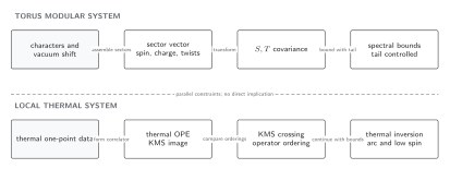
Thermal crossing begins with an ordered correlator on $S^1_\beta\times\mathbb R^{d-1}$. The OPE and its KMS image must overlap, image or spectral tails must be bounded, and inversion additionally needs a declared analytic sheet, growth exponent, spin range, and arc terms. The separate torus path concerns global two-dimensional sector traces. Schematic and not to scale.

The process and its failure checks are summarized semantically here:

Stage	Mathematical object	Exact domain or equality	Truncation or continuation check	Failure signal
State	$Z^{-1}e^{-\beta H}$	normalized trace in a specified ensemble	spectral tail must preserve the same normalization	identity expectation differs from one
Local OPE	sum over $a_{\mathcal O}$	$r<\beta$	bound undifferentiated and differentiated tails separately	cutoff drift grows near $r=\beta$
KMS image	reversed operator order	$G(\tau,\mathbf x)=G(\beta-\tau,-\mathbf x)$ for the identical bosonic scalar	include statistics or charge phase in other sectors	odd derivatives at $\beta/2$ remain nonzero beyond the tail bound
Image benchmark	sum over $m\in\mathbb Z$	absolute convergence for $\Delta_\phi>1/2$	use the explicit $M$-tail bound above	zero-mode or borderline logarithmic divergence
Thermal inversion	discontinuity of the continued correlator	only on the declared Lorentzian cut and above the growth-controlled spin threshold	retain arcs and low-spin terms when required	reconstructed coefficient changes under contour or cutoff refinement

From an equation to a numerical problem

A well-posed truncated KMS system records:

• spacetime dimension $d$ and external dimension $\Delta_\phi$;
• canonical, charged, or rotating ensemble;
• vacuum two-point and OPE normalizations;
• tensor basis and all symmetry selection rules;
• the common OPE domain for a point and its KMS image;
• image, descendant, and primary cutoffs with independent tail estimates; and
• the exact statistics or chemical-potential phase.

Because $a_{\mathcal O}$ is sign-indefinite, a small least-squares residual is evidence only for that truncation. It does not prove existence or uniqueness of a thermal state. Extra correlators, known vacuum OPE data, thermodynamic input, or inversion constraints can make the system more informative.

Scope beyond this page

The general theory of density matrices, KMS states, spectral functions, and the equilibrium-to-real-time interface continues in Thermal and Nonequilibrium QFT. This page uses those principles only to build the CFT-specific local OPE and crossing equation.

Common failure modes

Expanding outside the contractible ball. Periodicity of the full correlator does not make one local OPE convergent everywhere. Check both $r<\beta$ and $r'<\beta$.

Dropping the order reversal. KMS relates ordered products. For nonidentical or fermionic operators, writing simple periodicity loses essential data.

Imposing coefficient positivity. The thermal coefficient contains $f_{\phi\phi\mathcal O}b_{\mathcal O}$ and can have either sign.

Using an image cutoff without its tail. KMS can appear violated merely because the truncated set is not closed under $m\mapsto-m-1$. Compare the residual with the analytic tail bound.

Exercises

Show directly that the generalized-free image sum is KMS symmetric.

Solution

At the image point,

$$\beta-\tau+m\beta =-\left[\tau+(-m-1)\beta\right].$$

The square removes the sign, and $m\mapsto-m-1$ is a bijection of $\mathbb Z$. Therefore the full sum is unchanged. A symmetric finite cutoff is not exactly mapped to itself, which is why the omitted tail must accompany a truncated KMS check.

For $\Delta_\phi=1$ and $\tau=\beta/2$, bound the image tail after $\lvert m\rvert\le M$.

Solution

Here $u=1/2$ and $2\Delta_\phi-1=1$, so

$$\lvert R_M\rvert \le\frac{2}{\beta^2(M-1/2)}.$$

The bound is uniform in spatial separation and valid for $M>1/2$.

Continue to inversion

Thermal Inversion and Sum Rules turns the KMS correlator into pole data while keeping the analytic domain, discontinuity, arcs, and low-spin terms explicit.

A reproducible calculation should evaluate exact image sums at several $\beta$, vary the image cutoff independently of inversion precision, and require the analytic tail above.

References

• Iliesiu, Luca, Murat Koloğlu, Raghu Mahajan, Eric Perlmutter, and David Simmons-Duffin. “The Conformal Bootstrap at Finite Temperature.” Journal of High Energy Physics 2018, no. 10 (2018): 070. doi:10.1007/JHEP10(2018)070. Open preprint.