Sphere Partition Functions and Universal CFT Data

The sphere partition function packages a CFT’s response to curvature in one number, but that number is not universally meaningful in every dimension. In even dimensions the logarithmic radius dependence is controlled by the Euler anomaly while the finite part is counterterm dependent. In odd dimensions the real finite part can be universal under the usual locality and symmetry assumptions. Zero modes, gauge volumes, and source contacts must be treated before either statement is applied.

Required background. Anomaly Coefficients and Central Charges fixes type-A normalization. Weyl Covariance on Curved Backgrounds fixes the generating functional. Helpful background. Defect Entropy and Monotonicity compares sphere-like observables localized on a defect.

Radius response on a round sphere

Consider a CFT on a smooth closed round sphere of radius $r$, with the zero-mode measure fixed and local power-law terms subtracted. Keep the renormalization scale fixed when varying $r$, and reserve $R$ for scalar curvature. Define

$$F_{S^d}(r)=-\log Z[S^d_r]=W[S^d_r].$$

A constant change of radius is a Weyl rescaling. With the inherited positive covariant-metric variation of $W$,

$$\frac{dF_{S^d}}{d\log r} =\int_{S^d}d^dx\sqrt g\, \langle T^\mu{}_{\mu}\rangle.$$

For a nonchiral two-dimensional CFT with $c_L=c_R=c$ and $\langle T^\mu{}_{\mu}\rangle=-cR/(24\pi)$, the integral $\int_{S^2}\sqrt g\,R=8\pi$ gives $dF_{S^2}/d\log r=-c/3$. For the parity-even purely gravitational anomaly of a four-dimensional CFT,

$$\langle T^\mu{}_{\mu}\rangle =\frac{aE_4-cC^2+b_m\nabla^2R}{(4\pi)^2},$$

the round sphere has $C^2=0$, $\nabla^2R=0$, and $\int_{S^4}\sqrt g\,E_4=64\pi^2$, hence

$$\frac{dF_{S^4}}{d\log r}=4a.$$

These signs use the stress and positive $a,c$ normalization of the fixed-point trace calculation. In particular, a real conformal scalar has $a=1/360$ and sphere response $+1/90$ in four dimensions; its positive conformal Laplacian has no zero mode. The coefficient of $\log(r/r_0)$, with fixed reference radius $r_0$, is universal. A finite $r$-independent term can be shifted by allowed local curvature counterterms, while unsubtracted cosmological or Einstein terms would add separate powers of $r$.

Odd and even dimensions

The useful distinction is:

Dimension	Universal sphere datum on a closed sphere	Main qualification
Even $d$	coefficient of the logarithm, proportional to type-A data	finite part is scheme dependent
Odd $d$	real finite part $F=-\log\lvert Z\rvert$	parity-odd phases and topological counterterms are separate
Noninteger $d$ in an expansion	a chosen analytic continuation such as $\widetilde F$	continuation and subtraction convention must be stated

In three dimensions, the use of the real sphere free energy as an endpoint quantity and its perturbative tests are developed in Klebanov, Pufu, and Safdi 2011. This does not remove the zero-mode, phase, or endpoint qualifications stated here.

A frequently useful interpolation is

$$\widetilde F(d)=-\sin\!\left(\frac{\pi d}{2}\right)F_{S^d},$$

which connects odd-dimensional finite terms to even-dimensional anomaly residues in dimensional regularization Giombi and Klebanov 2015, §§1–2. Here one uses the chosen dimensionally continued expression before subtracting its even-dimensional pole. If

$$F_{S^d}=\frac{f_{-1}}{d-2n}+f_0+O(d-2n), \qquad \lim_{d\to2n}\widetilde F(d)=(-1)^{n+1}\frac\pi2 f_{-1}.$$

The limit follows by expanding the sine. A finite change of $f_0$ cannot change it. Continuation away from integer dimension and the finite subtraction still require a prescription; this interpolation by itself is not a dimension-independent monotonicity theorem.

Source derivatives and integrated correlators

At fixed background metric, introduce real constant sources $\lambda^I$ linearly in the Euclidean action, keeping the displayed operators fixed under this variation:

$$S\longmapsto S+\lambda^I\int_{S^d}\sqrt g\,\mathcal O_I.$$

Then

$$\partial_I F =\int_{S^d}\sqrt g\,\langle\mathcal O_I\rangle,$$

and

$$\partial_I\partial_JF =-\int_{S^d}\sqrt g_x\int_{S^d}\sqrt g_y\, \langle\mathcal O_I(x)\mathcal O_J(y)\rangle_{\!c} +\text{local counterterms}.$$

The negative connected term follows from the real action source $+\lambda^I\int\mathcal O_I$. If the operators or renormalized counterterms depend explicitly on $\lambda$, their source derivatives must also be retained as local contact contributions. Coincident-point singularities make the double integral regulator dependent; these contacts can alter the Hessian. On a conformal manifold, a protected combination can define the Zamolodchikov metric only after redundant directions and source coordinates are fixed.

Zero modes and normalization

A functional determinant with a zero eigenvalue is not defined by simply including that eigenvalue in $\log\det$. One must separate the zero modes and specify their integration or quotient and measure normalization. Examples include:

• the constant mode of a noncompact massless scalar;
• gauge transformations and ghost zero modes;
• Goldstone modes in a spontaneously broken description;
• collective coordinates around a saddle.

For the real noncompact massless scalar on $S^2$, let $A=4\pi r^2$ and define the metric-independent field volume $V_0=\int d\phi_0$ with a fixed field-value range. The normalized constant-mode coefficient is $a_0=\sqrt A\,\phi_0$, so dividing $\int da_0=\sqrt A\,V_0$ by $V_0$ leaves $\sqrt A$ in the partition function. The anomaly-normalized scalar free energy is therefore

$$F_{\rm scalar}=\frac12\log\frac{\det'(-\nabla^2)}{A},$$

up to constants fixed by the measure and renormalization units. It has the $c=1$ response $dF/d\log r=-1/3$; omitting the constant eigenfunction without the area factor gives a different scale dependence. The closed-surface scalar derivation explains the finite Weyl formula, using the determinant scaling in Sarnak 1990, §1, pp. 603–605, PDF. This scalar example is not a definition of an arbitrary interacting CFT or a prescription for gauge zero modes.

Different mode and quotient choices can add $\log r$ or volume factors. State them before evaluating the determinant and compare the scale derivative with the anomaly in the same normalization.

The anomaly-to-sphere branch of the Weyl response diagram has this structured equivalent:

Stage	Retain	Do not confuse with
Regulated determinant or path integral	regulator, measure, zero-mode prescription	renormalized $F$
Local subtraction	divergent and finite curvature counterterms	universal coefficient
Even-dimensional output	logarithmic coefficient	arbitrary finite constant
Odd-dimensional output	real finite part in a symmetry-preserving scheme	parity-odd phase
Source differentiation	integrated connected correlator plus contacts	separated-point correlator alone

The sphere box uses the renormalized generating functional and its local-response information (W + B), with fixed-point and measure assumptions stated explicitly. Follow the dashed endpoint arrow only when the hypotheses of the relevant flow theorem also hold.

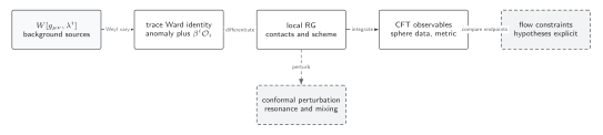
At a conformal fixed point, universal sphere data require controlled local subtraction, measure normalization and zero-mode treatment. The appropriate even-dimensional logarithmic term or odd-dimensional real finite part is selected as described above. Here $W=-\log Z$, $T$ is the positive covariant-metric source response, and $\beta_\mu^I=\mu\,dg^I/d\mu$; the local trace therefore contains the anomaly minus the beta–operator term. The sphere calculation does not require passing through conformal perturbation, and endpoint comparison alone does not prove monotonicity. Schematic, not to scale.

Comparing sphere calculations

To compare sphere calculations, specify the spectrum or integrand, regulator, counterterm basis, zero-mode measure, numerical precision and radius convention, and verify the scale derivative. The raw number $-\log Z$ without those data is not comparable across methods.

Common pitfalls

Calling the even-dimensional finite part universal. A finite local curvature counterterm shifts it. The logarithmic coefficient is the invariant datum.

Deleting zero modes silently. Their measure and physical quotient can contribute scale dependence. State the treatment before evaluating the determinant.

Equating a source Hessian with an ordinary integrated two-point function. Coincident singularities generate local terms. The metric or susceptibility is defined only after a subtraction and coordinate convention.

Exercises

Derive $dF_{S^4}/d\log r=4a$ in the convention above.

Solution

The round sphere is conformally flat and has constant scalar curvature, so only $aE_4/(4\pi)^2$ contributes. Since $\int_{S^4}\sqrt gE_4=32\pi^2\chi(S^4)=64\pi^2$, the integral is $a(64\pi^2)/(16\pi^2)=4a$.

References

• Giombi, S., and Klebanov, I. R. “Interpolating between $a$ and $F$.” Journal of High Energy Physics 2015, 117 (2015). arXiv. DOI.

• Klebanov, I. R., Pufu, S. S., and Safdi, B. R. “F-Theorem without Supersymmetry.” Journal of High Energy Physics 2011, 038 (2011). arXiv. DOI.

• Sarnak, P. “Determinants of Laplacians; Heights and Finiteness.” In Analysis, et cetera, edited by P. H. Rabinowitz and E. Zehnder, 601–622. Academic Press, 1990. Open PDF.

Further reading

• Pufu, S. S. “The F-Theorem and F-Maximization.” Journal of Physics A 50, 443008 (2017). arXiv. DOI.