Conformal Perturbation Theory and Beta Functions

Conformal perturbation theory computes the initial motion away from a CFT using its operator dimensions, OPE coefficients, and integrated correlators. Ultraviolet collisions of insertions generate beta functions, anomalous dimensions, and mixing. The calculation is predictive only after the operator normalization, cutoff, contact terms, and subtraction scheme have been stated. A CFT derivation of this strategy near the Wilson–Fisher fixed point appears in Rychkov and Tan 2015, §§2–3.

Required background. Local RG and Weyl Consistency Conditions supplies source covariance and scheme changes. Conformal OPE Data fixes dimensions and OPE coefficients. Helpful background. Operator Mixing and Renormalization Matrices supplies the matrix treatment of degenerate operators.

Perturbing a fixed point

Choose unit-normalized scalar primaries $\mathcal O_i$ and write

$$S=S_{\rm CFT} +\sum_i g^i\mu^{d-\Delta_i} \int d^dx\,\mathcal O_i(x).$$

The $g^i$ are dimensionless and

$$\mu\frac{dg^i}{d\mu} =(\Delta_i-d)g^i+O(g^2).$$

Thus a relevant coupling grows toward the infrared. This linear term is invariant under analytic redefinitions that preserve the fixed point; the relation between scaling dimensions and the linearized RG flow is developed in Cardy 1996, chs. 5 and 9.

At second order, two insertions collide. In the normalization

$$\mathcal O_j(x)\mathcal O_k(0) \sim\sum_i \frac{C_{jk}{}^i}{|x|^{\Delta_j+\Delta_k-\Delta_i}} \mathcal O_i(0)+\cdots,$$

a logarithm appears when $\Delta_j+\Delta_k-\Delta_i=d$. For nearly marginal scalars in a hard-sphere minimal subtraction convention,

$$\beta^i=(\Delta_i-d)g^i +\frac{S_{d-1}}{2}C_{jk}{}^i g^jg^k +O(g^3), \qquad S_{d-1}=\frac{2\pi^{d/2}}{\Gamma(d/2)}.$$

The factor $1/2$ compensates the exchange of the two integrated insertions. Changing the sign of the deformation in $S$, the normalization of $\mathcal O_i$, or the subtraction convention changes the displayed quadratic coefficient coherently. The derivation—not the bare formula—is what should be transported between conventions. For marginal deformations, the same contact terms furnish connection data on coupling space and cannot generally be set to zero in every chart Kutasov 1989.

For one nearly marginal coupling with $\Delta=d-\epsilon$,

$$\beta(g)=-\epsilon g+\frac{S_{d-1}}{2}C_{\mathcal O\mathcal O}{}^{\mathcal O}g^2+O(g^3).$$

If the quadratic coefficient is positive, the perturbative fixed point is

$$g_*=\frac{2\epsilon}{S_{d-1}C_{\mathcal O\mathcal O}{}^{\mathcal O}}+O(\epsilon^2).$$

This location is scheme dependent beyond the controlled order. Critical exponents evaluated consistently at $g_*$ can be scheme independent to that order.

Anomalous dimensions and mixing

Let the operators form a closed column and share quantum numbers. Use the bare-to-renormalized convention of Operator Anomalous-Dimension Matrices. With $\mathcal D=\mu\,d/d\mu|_0$ the total RG derivative at fixed bare data,

$$\begin{aligned} \mathcal X_{0,A}&=Z_A{}^B[\mathcal X_B], \\ \gamma_A{}^B&=(Z^{-1}\mathcal D Z)_A{}^B, \qquad \mathcal D[\mathcal X_A]=-\gamma_A{}^B[\mathcal X_B]. \end{aligned}$$

Indeed, $0=\mathcal D\mathcal X_0=(\mathcal D Z)[\mathcal X]+Z\mathcal D[\mathcal X]$; multiplying from the left by $Z^{-1}$ gives the displayed sign and matrix order. The derivative includes the running couplings. Reversing the defining direction of $Z$ requires changing the anomalous-dimension formula as well.

The logarithmic divergence of

$$-g^i\mu^{d-\Delta_i}\int d^dx\, \langle\mathcal X_A(x_1)\mathcal O_i(x)\mathcal X_B(x_2)\rangle$$

determines the leading mixing matrix. Individual diagonal entries depend on basis; eigenvalues at a fixed point are the anomalous dimensions of scaling operators. When dimensions are degenerate at zeroth order, diagonalize the full matrix with the two-point metric rather than correcting each operator independently.

A resonance occurs when dimensions make an integrated OPE term logarithmic. Power divergences are more scheme dependent, while logarithms control universal leading running in the stated basis. Descendants, total derivatives, and redundant operators must be quotiented before interpreting the spectrum.

Integrated-correlator workflow

1. Normalize all two-point functions and OPE coefficients at the reference CFT.
2. Excise balls of radius $a$ around every collision, or declare an equivalent regulator.
3. Insert the OPE in each collision region and integrate angular factors.
4. Add the complete local counterterm basis, including source and curvature terms.
5. Differentiate bare couplings at fixed bare data to obtain $\beta^i$ and $\gamma_A{}^B$.
6. Check permutation factors and overlapping subdivergences.
7. Repeat after a coupling or operator-basis change; invariant predictions must agree.

The two source branches distinguish normalized fixed-point OPE data (A) from local response and subtraction choices (B). The conformal-perturbation box uses both inputs; the sphere calculation is a separate application of the generating functional.

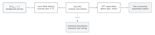
Conformal perturbation combines normalized fixed-point CFT correlators with regulated coincidence regions and local counterterms. Basis, scheme and truncation errors must be controlled before interpreting invariant predictions. In the local-response branch, $W=-\log Z$, $T$ is the positive covariant-metric source response, and $\beta_\mu^I=\mu\,dg^I/d\mu$; this fixes the minus-beta trace term. The sphere and flow boxes are distinct, qualified applications rather than subsequent steps of every perturbative calculation. Schematic, not to scale.

Its deformation branch has the following structured equivalent:

Input	Operation	Output	Required control
$\Delta_i$	dimensional analysis	linear beta term	source normalization
$C_{jk}{}^i$	integrate resonant OPE singularity	quadratic beta term	angular factor and permutation
$\langle\mathcal X_A\mathcal O_i\mathcal X_B\rangle$	extract logarithmic mixing	$\gamma_A{}^B$	two-point metric and degeneracy
Local source terms	subtract coincident regions	scheme choice	complete counterterm basis
Perturbative zero of $\beta$	evaluate invariant observables	fixed-point exponents	order and remainder estimate

Reproducible checks

A reproducible benchmark should separate source contacts from universal response. It must expose the regulator, counterterms, truncation order, precision, and a deliberately wrong OPE normalization that fails its checks.

Common pitfalls

Reading a power divergence as a universal beta coefficient. Universal leading running comes from the logarithmic collision after the scheme is fixed. Power subtractions are more regulator dependent.

Ignoring degenerate mixing. A diagonal correction in an arbitrary basis is not a scaling dimension. Solve the generalized eigenvalue problem using the two-point metric.

Quoting $g_*$ more accurately than the beta function. A fixed point found at $O(\epsilon)$ has an $O(\epsilon^2)$ uncertainty unless the next order is computed.

Exercises

Derive the factor $S_{d-1}/2$ in the quadratic beta function for identical perturbing operators.

Solution

The second-order expansion supplies $g^2/2$. In the resonant OPE channel the relative-coordinate integral is $\int_a dr\,r^{d-1}r^{-d}=\log(1/a)$, while the angular integral is $S_{d-1}$. Multiplying by $C_{\mathcal O\mathcal O}{}^{\mathcal O}$ gives the stated coefficient in the declared subtraction convention.

References

• Cardy, J. Scaling and Renormalization in Statistical Physics. Cambridge Lecture Notes in Physics 5. Cambridge University Press, 1996, chs. 5 and 9. Publisher.
• Kutasov, D. “Geometry on the Space of Conformal Field Theories and Contact Terms.” Physics Letters B 220 (1989): 153–158. DOI.
• Rychkov, S., and Tan, Z. M. “The $\epsilon$-Expansion from Conformal Field Theory.” Journal of Physics A 48, 29FT01 (2015). arXiv. DOI.