Strong Hyperbolicity, Stability, and Causal Propagation

A damped dispersion relation is evidence about a linearized solution in one background; it is not, by itself, a proof of causal propagation or of a well-posed nonlinear initial-value problem. Those conclusions belong to a hierarchy. Causality is controlled by the principal characteristics, strong hyperbolicity by their uniformly complete eigensystem, local existence by an energy estimate plus regularity and compatibility hypotheses, and nonlinear stability or shock admissibility by still stronger arguments.

Required background. Israel–Stewart-Type Transient Hydrodynamics supplies a relaxation system whose modes can be checked explicitly. BDNK First-Order Causal Hydrodynamics gives a relativistic example in which a coefficient domain controls the full principal symbol.

Helpful background. Weak Solutions, Sobolev Spaces, and Well-Posedness develops the function-space statements used below.

Seven questions that must not be conflated

For a quasilinear first-order system

$$A^0(U,x)\,\partial_tU+A^i(U,x)\,\partial_iU=F(U,x),$$

each row below asks a different question.

Claim	Object to inspect	A positive result means	It does not yet mean
Linear mode stability	Roots $\omega_a(\mathbf k)$ about a specified background	$\operatorname{Im}\omega_a\le 0$ in the declared Fourier convention	Causality, diagonalizability, or nonlinear stability
Group velocity	$\partial\operatorname{Re}\omega_a/\partial k$ for a wave packet	Motion of a packet peak in a regime where that packet construction applies	A rigorous signal cone in a dissipative medium
Front velocity	The large-frequency edge of the retarded response	The speed of a sufficiently sharp disturbance under suitable analyticity hypotheses	Strong hyperbolicity of a general variable-coefficient system
Characteristic causality	$\det(A^\mu\xi_\mu)=0$	The local PDE characteristic cone lies within the metric light cone	Existence, uniqueness, or stability
Strong hyperbolicity	Principal eigenvalues and eigenvectors for every spatial direction	A uniform high-frequency energy estimate for the linearized principal system	A global nonlinear solution or shock admissibility
Local well-posedness	A quasilinear energy estimate in a stated function space	Short-time existence, uniqueness, and continuous dependence	Global existence, decay, or absence of singularities
Nonlinear stability and weak continuation	Nonlinear norm estimates and an admissibility criterion	Persistence near a background, or a selected continuation after breakdown	A conclusion that follows from rest-frame damping alone

The relativistic hydrodynamic consistency reference records this separation across the main fluid frameworks.

The framework map below applies the same discipline to four alternative formulation families. Read vertically rather than horizontally: each family has its own independent stability, spectrum, closure, and hyperbolicity question.

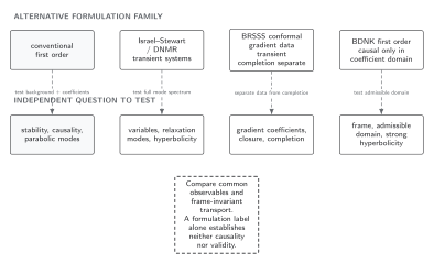
No formulation name establishes causality or well-posedness. Conventional first order, transient Israel–Stewart or DNMR systems, BRSSS gradient data with a separately chosen completion, and BDNK in an admissible coefficient domain require different principal and lower-derivative checks. The diagram compares parallel alternatives and is not a hierarchy of increasing validity.

In text: fix the physical tensors and common infrared transport, declare the variables and exact truncation, calculate the full mode spectrum and principal symbol, and state the coefficient, background, and regularity domain. Only then can stability, causality, or strong hyperbolicity be attached to that particular formulation.

Modes retain lower-derivative physics

Freeze a homogeneous background $U_0$ and insert the site convention

$$\delta U=\widehat U\,e^{-i\omega t+i\mathbf k\cdot\mathbf x}.$$

The complete linear dispersion relation is

$$\det\!\left[-i\omega A^0(U_0)+ik_iA^i(U_0)-B(U_0)\right]=0,$$

where $B=\partial F/\partial U$ after moving all terms to the same side. The matrix $B$ controls relaxation and other lower-derivative effects. It can damp or amplify modes, but it does not change the characteristic polynomial of the principal part.

Linear stability therefore requires the full roots at real $\mathbf k$, not merely their small-$k$ expansions. It must also be tested about every background in the claimed state domain. In a Lorentz-covariant dissipative theory, a rest-frame test alone can miss instabilities seen by boosted observers; Hiscock and Lindblom’s analysis of conventional relativistic dissipative fluids is the classic warning Hiscock and Lindblom 1985, §§II–IV, pp. 726–731.

Nor is group velocity a substitute for causality. Near a collision of damped branches, $\partial_k\operatorname{Re}\omega$ can be singular or superluminal even when the characteristic cone is subluminal. Conversely, a parabolic diffusion root has no finite front at all despite its innocuous small-$k$ damping. Signal propagation is a high-frequency, initial-value question.

Principal symbols and hyperbolicity

For a covector $\xi_\mu$, define

$$P(\xi)=A^\mu\xi_\mu.$$

A hypersurface with normal $\xi_\mu$ is characteristic when $\det P(\xi)=0$. Given a time covector for which $A^0$ is invertible, the directional evolution matrix is

$$M(\mathbf n)=(A^0)^{-1}A^i n_i, \qquad \mathbf n^2=1.$$

Weak hyperbolicity asks only that the eigenvalues of $M(\mathbf n)$ be real. That is insufficient: a repeated eigenvalue with a Jordan block produces polynomial growth proportional to powers of $k t$ and destroys a derivative-preserving estimate.

Strong hyperbolicity additionally requires a complete eigenbasis whose condition number is bounded uniformly over all directions $\mathbf n$ and all states in the domain under study. Equivalently, under standard smoothness assumptions, there is a positive directional symmetrizer $H(\mathbf n)$ with uniform upper and lower bounds. Symmetric hyperbolicity is stronger: a single positive matrix $H(U,x)$ makes $HA^0$ positive and every $HA^i$ symmetric. Symmetric systems admit direct energy estimates; strong systems generally require a frequency-dependent construction. Reula gives a concise account of these distinctions and their role in the Cauchy problem Reula 1998, §§2–3, pp. 1–12, Open PDF.

For relativistic hydrodynamics, characteristic causality then asks that every characteristic speed measured in every local fluid rest frame satisfy

$$\lvert v_{\mathrm{char}}\rvert\le 1.$$

This is classical domain-of-dependence causality for the effective PDE. It is not the microscopic QFT statement that spacelike commutators vanish, and it is credible only below the theory’s ultraviolet cutoff.

Complete check of a relaxation model

Consider a conserved scalar density coupled to a relaxing spatial current in $d$ dimensions:

$$\partial_t n+\partial_i j^i=0, \qquad \tau\,\partial_tj_i+D\,\partial_i n=-j_i,$$

with constants $D>0$ and $\tau>0$. This is the covariant channel structure behind the simplest Maxwell–Cattaneo or Israel–Stewart diffusion sector, evaluated in a homogeneous rest frame.

For a wavevector $\mathbf k=k\mathbf n$, the longitudinal determinant gives

$$\tau\omega^2+i\omega-Dk^2=0,$$

and hence

$$\omega_\pm(k) = \frac{-i\pm\sqrt{4\tau Dk^2-1}}{2\tau}.$$

At small $k$, one branch is hydrodynamic and the other transient:

$$\omega_{\mathrm{hyd}}=-iDk^2+O(k^4), \qquad \omega_{\mathrm{tr}}=-\frac{i}{\tau}+iDk^2+O(k^4).$$

Both have nonpositive imaginary part for every real $k$. At large $k$,

$$\omega_\pm = \pm\sqrt{\frac{D}{\tau}}\,k-\frac{i}{2\tau}+O(k^{-1}),$$

so the front speed is $\sqrt{D/\tau}$.

The principal-symbol check is independent and stronger. With $U=(n,j_1,\ldots,j_d)^T$, the directional matrix has a longitudinal block

$$M_{\parallel}(\mathbf n) = \begin{pmatrix} 0&1\\[2pt] D/\tau&0 \end{pmatrix}$$

and $d-1$ transverse zero eigenvalues. Its eigenvalues are

$$v_\pm=\pm\sqrt{\frac{D}{\tau}}, \qquad v_{\perp}=0,$$

with a complete basis for every $\mathbf n$. A direction-independent positive symmetrizer is

$$H=\operatorname{diag}\!\left(\frac{D}{\tau},1,\ldots,1\right),$$

because $HM(\mathbf n)$ is symmetric. Thus this constant-coefficient model is symmetric hyperbolic, and its characteristic cone is inside the metric light cone precisely when

$$0<\frac{D}{\tau}\le1.$$

The calculation has now established rest-frame damping, a complete eigensystem in every direction, an explicit symmetrizer, and a subluminal principal cone. It has not established a nonlinear theorem for state-dependent $D$ and $\tau$, compatibility with a particular physical boundary, or a weak solution after gradient blowup. Those require new hypotheses.

From the frozen symbol to a nonlinear theorem

For a quasilinear fluid, the following items must be supplied rather than inferred:

1. State domain. Temperature, enthalpy, and transport coefficients must remain in a region where $A^0$ and the symmetrizer are uniformly positive.
2. Coefficient regularity. The equation of state and transport functions need the differentiability required by the energy estimate.
3. Initial data and constraints. Velocity normalization, conserved-charge constraints, and any auxiliary first-order-reduction constraints must hold initially and propagate.
4. Function space. A theorem might use $H^s$ with $s>d/2+1$, Gevrey data, or another class. The exact threshold is theorem-specific.
5. Boundaries. On a domain with boundary, incoming characteristic fields require maximally dissipative or otherwise compatible data. A periodic-domain proof does not supply them.
6. Uniformity. Eigenvectors that become singular at an admissible state boundary invalidate a uniform estimate even if the eigenvalues remain real there.

The conformal BDNK Sobolev theorem, for example, fixes the background spacetime and spatial topology, regularity, positivity, and coefficient inequalities; the general BDNK theorem supplies a different hypothesis set for charged, nonconformal fluids Bemfica et al. 2021, Theorem 1.1, pp. 2281–2283 and Bemfica, Disconzi, and Noronha 2022, Theorems I–III, pp. 18–29, Open PDF. Quoting either theorem without its hypotheses overstates the result.

Nonlinear stability, breakdown, and shocks

Local well-posedness says that nearby admissible initial data produce nearby solutions for a common short time. Nonlinear stability of an equilibrium is stronger: it normally requires a norm that stays controlled, often with decay, for all future time for sufficiently small perturbations. A linear spectrum is an ingredient in such a proof, not the proof itself; nonlinear couplings, derivative loss, zero modes, boundaries, and the state-domain edge can all intervene.

Even symmetric-hyperbolic ideal relativistic Euler equations can develop shocks from smooth compressive data. At that point the classical solution ends although the characteristic speeds were causal before breakdown. Continuing with a weak solution requires conservation in the distributional sense plus an entropy or other admissibility condition. Viscous or transient theories pose different questions: one must prove existence of a shock profile, stability of that profile, and convergence in the intended regulator limit. None follows from a homogeneous dispersion plot.

Accordingly, the strongest defensible statement should name its ceiling. “Stable linear modes about global equilibrium,” “causal and strongly hyperbolic on this coefficient domain,” “locally well posed in this Sobolev class,” and “globally nonlinearly stable for small data” are not stylistic variants; they are distinct results.

Reproducible consistency checklist

For any proposed relativistic fluid PDE, record:

• the metric, Fourier sign, hydrodynamic frame, background state, and coefficient domain;
• all dispersion roots for real wavevectors, including nonhydrodynamic branches and boosted backgrounds;
• the principal characteristic polynomial for every spatial direction;
• degeneracy surfaces, eigenvector completeness, and uniform bounds or an explicit symmetrizer;
• comparison of every characteristic cone with the metric light cone;
• constraints and their propagation equations;
• coefficient regularity, initial-data space, and the exact local-existence theorem used;
• boundary conditions classified by incoming characteristics;
• the nonlinear norm and time interval of any stability claim;
• the weak-solution and entropy criterion if shocks are admitted;
• the effective-theory cutoff beyond which high-frequency conclusions are not physical.

A reproducible calculation can be used for reconstructing spectra and scanning characteristic speeds. Numerical scans are valuable adversarial evidence, but a finite grid of states and directions cannot prove uniform diagonalizability.

The next diagram makes the logical independence of the main diagnostics spatially explicit. Inspect the four solid spokes from the declared theory and background, then the dashed spoke to the observable hydrodynamization criterion.

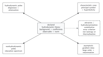
Hydrodynamic dispersion, characteristic causality and hyperbolicity, nonhydrodynamic relaxation, and large-order asymptotics are independent outputs of a fully declared theory and background. An attractor or hydrodynamization statement additionally requires an observable, norm, and error tolerance, and does not imply isotropy or thermalization. The diagram is a logical map, not a temporal sequence.

In text: the full linear operator determines hydrodynamic and transient poles; the principal symbol alone determines characteristics; a nonlinear expansion supplies large-order data; and comparison with time-dependent solutions supplies a bounded hydrodynamization criterion. None of these calculations can be substituted for another.

Exercise

Set $D=1/3$ and $\tau=1/2$ in the relaxation model. Establish linear stability, find the characteristic speeds and a symmetrizer, and state the strongest conclusion that follows.

Solution

The roots are

$$\omega_\pm = -i\pm\sqrt{\frac{2}{3}k^2-1},$$

where the square root is either real or purely imaginary. For small $k$, both roots lie on the nonpositive imaginary axis; after the branch collision they have imaginary part $-1$. Thus the homogeneous constant-coefficient model is linearly stable.

The characteristic speeds are

$$v_\pm=\pm\sqrt{\frac{2}{3}},$$

and the transverse speeds are zero. One may take

$$H=\operatorname{diag}\!\left(\frac{2}{3},1,\ldots,1\right).$$

The model is therefore symmetric hyperbolic and its principal cone is subluminal. This proves a well-posed constant-coefficient linear Cauchy problem with finite propagation speed. It does not prove a quasilinear theorem, boundary well-posedness, nonlinear stability, or shock admissibility.

Common pitfalls

Using $\operatorname{Im}\omega\le0$ as a causality test. Damping concerns time dependence; causality concerns the principal domain of dependence. Diffusion is damped and acausal.

Checking eigenvalues but not eigenvectors. Real characteristic speeds with a Jordan block give weak, not strong, hyperbolicity.

Treating a group-velocity spike as a superluminal signal. In a dissipative system, the packet peak need not track the front. Inspect characteristics and the retarded support.

Calling local existence nonlinear stability. A short-time solution may later leave the admissible state domain or form a singularity.

Where this leads

Hydrodynamic Attractors and Asymptotic Gradient Expansions asks how transient modes govern approach to a hydrodynamic slow manifold. It uses the hierarchy here to keep rapid hydrodynamization distinct from a global nonlinear theorem.

References

• Bemfica, Fábio S., Marcelo M. Disconzi, and Jorge Noronha. 2022. “First-Order General-Relativistic Viscous Fluid Dynamics.” Physical Review X 12: 021044. DOI. Open PDF.

• Bemfica, Fábio S., Marcelo M. Disconzi, Casey Rodriguez, and Yuanzhen Shao. 2021. “Local Existence and Uniqueness in Sobolev Spaces for First-Order Conformal Causal Relativistic Viscous Hydrodynamics.” Communications on Pure and Applied Analysis 20: 2279–2290. DOI. Open PDF.

• Hiscock, William A., and Lee Lindblom. 1985. “Generic Instabilities in First-Order Dissipative Relativistic Fluid Theories.” Physical Review D 31: 725–733. DOI.

• Reula, Oscar A. 1998. “Hyperbolic Methods for Einstein’s Equations.” Living Reviews in Relativity 1: 3. DOI. Open PDF.