Lyapunov Growth and Chaos Bounds

The thermal chaos bound is a complex-analysis theorem for a normalized, regularized OTOC that is analytic and bounded in a half-strip and has a parametrically small connected correction over a dissipation-to-scrambling window. Under those hypotheses, an exponential correction cannot grow faster than $2\pi/\beta$. It is not a bound on every squared commutator, every classical Lyapunov exponent, or every exponential fitted in a finite system.

Required background. OTOCs and contour regularization fixes the correlator and its thermal contour. Holomorphic functions and Cauchy theory supplies the maximum-modulus and Schwarz–Pick tools. Helpful background. Late-time spectral evidence provides an independent chaos diagnostic with different assumptions.

The theorem’s correlator and hypotheses

Let $y^4=\rho_\beta$ and consider bounded Hermitian operators $V,W$. A symmetric thermal OTOC is

$$F(t)=\operatorname{Tr}\left[yVyW(t)yVyW(t)\right].$$

Normalize it by a positive disconnected scale $F_d$ and write

$$f(t)=\frac{F(t)}{F_d} =1-\varepsilon e^{\lambda t}+\cdots, \qquad 0<\varepsilon e^{\lambda t}\ll1.$$

The Maldacena–Shenker–Stanford argument requires, in the relevant time range:

1. analyticity of the continued normalized correlator in the thermal half-strip;
2. a bound $\lvert f\rvert\le1$ on its boundaries, up to controlled small corrections;
3. a positive normalization and factorized/disconnected reference;
4. a time $t_d$ after ordinary dissipation transients;
5. a later time $t_*$ before the connected correction becomes order one; and
6. enough separation that the exponential rate is meaningful rather than a local fit.

Then

$$\lambda\le\frac{2\pi}{\beta}$$

in units $\hbar=k_{\mathrm B}=1$ Maldacena, Shenker, and Stanford 2016, §§2–4.

Why strip analyticity fixes the rate

The proof maps the thermal half-strip conformally to the unit disk. If $z$ is the strip coordinate and $w(z)$ is the mapped bounded correlator, the Schwarz–Pick inequality constrains

$$\frac{\lvert w'(z)\rvert}{1-\lvert w(z)\rvert^2}$$

by the corresponding hyperbolic metric of the strip. On the real-time boundary and sufficiently far from the initial edge, this yields a differential inequality of the form

$$\frac{1}{1-f(t)}\left\lvert\frac{\mathrm d f}{\mathrm dt}\right\rvert \le \frac{2\pi}{\beta}+\text{controlled corrections}.$$

Substituting $1-f=\varepsilon e^{\lambda t}$ gives the rate bound. The number $2\pi/\beta$ is therefore set by the width of the analytic thermal strip, not by dimensional analysis alone.

This proof also explains the fragility of careless generalization. Change the density-matrix placement, lose the boundary bound, use unbounded unsmeared operators, or enter a regime where the connected piece is no longer small, and the theorem no longer applies in this form.

Fitting a rate is a separate inference problem

Suppose data for a connected correction $g(t)=1-f(t)$ are available. Compare at least

$$g_{\exp}(t)=Ae^{\lambda t}, \qquad g_{\mathrm{pow}}(t)=B(t-t_0)^p,$$

and a saturating form such as

$$g_{\mathrm{sat}}(t) =\frac{Ae^{\lambda t}} {1+Ae^{\lambda t}/g_\infty}.$$

Fit the full covariance, vary both window endpoints, and require a stable interval satisfying $g\ll1$ and $t>t_d$. A rate that changes when one point is removed is not resolved. If $t_*-t_d$ does not grow in the proposed large parameter or scaling limit, the word “Lyapunov” is descriptive rather than parametrically controlled.

For spatially separated operators, a form

$$g(t,x)\sim \exp\!\left[\lambda(v)t-\mu x\right]$$

can define velocity-dependent growth in some regimes. The thermal bound constrains a correlator under its analytic hypotheses; it does not equate the coefficient with the butterfly velocity or guarantee one universal front shape.

Regularization independence is an additional test

Different thermal placements can produce different early-time behavior. Tsuji, Shitara, and Ueda 2018 prove a rate bound for a family of regularized OTOCs when transient exponential growth occurs for every member and the inferred exponent is regularization independent. This is stronger than finding one convenient contour with a steep fit.

The practical test is therefore:

• compute at least two physically justified regularizations;
• translate their normalizations and disconnected pieces exactly;
• locate a common window rather than tuning separate ones; and
• treat exponent disagreement as evidence that the asymptotic regime has not been isolated.

Evidence ceiling and counterexamples

The theorem does not assert that a bound-saturating system exists, that saturation implies a unique microscopic mechanism, or that a system below the bound is chaotic. Integrable and free systems obey the bound trivially without showing a controlled exponential. Finite-dimensional systems can mimic exponentials across narrow windows. Classical systems can have Lyapunov exponents without a thermal OTOC satisfying the quantum hypotheses.

Conversely, a physically chaotic system may lack a clean exponential because no large parameter separates $t_d$ and $t_*$. Spectral statistics, operator fronts, transport, and ETH may still provide evidence. Use the thermalization and chaos evidence matrix to keep these conclusions distinct.

Common failure modes

Quoting the inequality without the correlator. State the density-matrix placement, normalization, operator domain, and analytic strip.

Treating the fit as the theorem. First establish the theorem’s hypotheses; then infer a rate with covariance and window stability.

Using saturation data. The derivation assumes the connected correction is small.

Identifying saturation with holography. A field-theory rate at the bound does not by itself establish a gravity dual; that comparison belongs to the holographic treatment.

Read the lower row as a set of distinct checks on a proposed exponential OTOC window: define the operator front and contour, fit only a controlled interval, test the bound’s hypotheses, and compare independent spectral evidence.

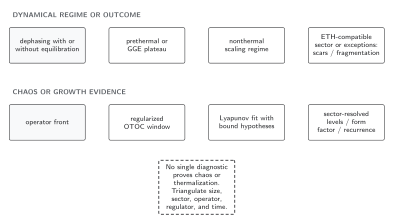
A fitted growth rate is conditional on operator choice, contour regularization, spatial regime, and a window separated from both dissipation and saturation. The bound applies only when its thermal analyticity assumptions hold. The diagram is schematic and its lower row has no implication arrows: spectral agreement can corroborate chaos but cannot prove the bound.

The text equivalent is a four-part test: specify the regulated OTOC, show a stable exponential interval, verify every hypothesis entering the bound, and vary size, operator, sector, and fit window. Spectral statistics can corroborate chaotic behavior but do not determine the same Lyapunov exponent.

Exercises

Insert $f(t)=1-\varepsilon e^{\lambda t}$ into the differential inequality and derive the bound.

Solution

$\lvert f'\rvert/(1-f)=\lambda$ while the exponential approximation holds. The strip inequality therefore gives $\lambda\le2\pi/\beta$ up to the controlled correction terms.

A fitted rate is $2.3\pi/\beta$ in a three-point window, but drops to $1.7\pi/\beta$ after including one earlier point. What is established?

Solution

No stable exponential rate is resolved, so there is neither a violation nor a confirmed test of the bound. Report window instability, examine alternative forms and regularizations, and seek a scaling limit that enlarges the interval.

Continue to spatial and spectral evidence

Operator spreading distinguishes the front velocity and broadening from the temporal exponent. Spectral form factors test late-time correlations without the OTOC strip hypothesis. Holographic saturation mechanisms continue in Volume XV.

References

• Maldacena, Juan, Stephen H. Shenker, and Douglas Stanford. “A Bound on Chaos.” Journal of High Energy Physics 2016, no. 8 (2016): 106. doi:10.1007/JHEP08(2016)106. Open preprint.
• Tsuji, Naoto, Tomohiro Shitara, and Masahito Ueda. “Bound on the Exponential Growth Rate of Out-of-Time-Ordered Correlators.” Physical Review E 98 (2018): 012216. doi:10.1103/PhysRevE.98.012216. Open preprint.