Unitarity, Normalization, and Largest-Time Identities

Microscopic unitarity constrains a closed-time-path theory more strongly than ordinary Hermiticity: equal histories cancel, so $Z[J,J]=1$ for every source profile. In the $r/a$ basis this forces the action to vanish at $\phi_a=0$, eliminates correlators whose strictly latest insertion is an $a$ field, and supplies practical normalization tests for regulators and approximations.

Required background. Use the closed-time-path generating functional and the distinction between unitary evolution and Hilbert-space positivity.

Helpful background. Trace, positivity, and causal consistency in open QFT shows how these conditions change after degrees of freedom are traced out.

Three exact identities

For a normalized $\rho_0$ and Hermitian Hamiltonian,

$$Z[J_+,J_-]=\operatorname{Tr}(U_{J_+}\rho_0U_{J_-}^\dagger)$$

obeys:

$$Z[J,J]=1, \qquad Z[J_+,J_-]^*=Z[J_-,J_+], \qquad Z[0,0]=1.$$

The first uses unitarity and trace cyclicity, the second Hermiticity, and the third also uses state normalization. A regulator or effective description must preserve the appropriate version of all three. An anomaly can modify a classical symmetry identity, but it does not license failure of trace normalization for a closed unitary system.

With $Z=e^{iW}$ and the chapter’s source rotation, equal sources mean $J_a=0$. The corresponding Schwinger–Keldysh normalization constraints are organized in Crossley, Glorioso, and Liu 2017, § 2. Therefore

$$W[J_r,J_a=0]=0, \qquad \left.\frac{\delta^nW}{\delta J_r(x_1)\cdots\delta J_r(x_n)}\right|_{J_a=0}=0.$$

Because $J_r$ couples to $\phi_a$, pure $a$ correlators vanish. Legendre transformation gives the corresponding effective-action condition

$$\Gamma[\phi_r,\phi_a=0]=0.$$

Thus every local term in a closed-system Schwinger–Keldysh effective action contains at least one $a$ field. This is normalization, not a claim that every coefficient is positive.

Largest-time identity

Consider a contour correlator expanded as a sum over branch assignments. If an insertion at the strictly latest time is changed from $+$ to $-$, all later forward and backward evolution has already cancelled; the two terms are equal up to the branch sign. Their difference—the $a$ insertion—vanishes. Hence

$$\langle\phi_a(t_{\max})\,\mathcal O_{r/a}(t_i<t_{\max})\rangle=0,$$

apart from specified equal-time contact terms. At two points,

$$-i\langle\phi_r(x)\phi_a(y)\rangle=G^R(x,y), \qquad -i\langle\phi_a(x)\phi_r(y)\rangle=G^A(x,y).$$

If the $a$ time is latest, both causal functions vanish. This is the causal content of the largest-time equation.

Equal times require care. Canonical commutators and derivative couplings can generate contact terms, while a lattice time contour requires a definite placement prescription. One must not infer that a nonzero equal-time response violates unitarity before accounting for these terms.

The dashed branch in the schematic is the generating identity from which the $a$-field selection rules follow. The final box combines two universal closed-system checks with one conditional equilibrium check; they should not be conflated.

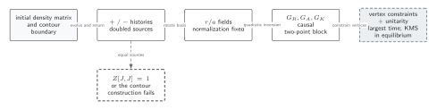
For normalized unitary evolution, equal branch sources give $Z[J,J]=1$, every connected all-$a$ correlator vanishes, and the largest-time identity removes a correlator whose latest insertion is an $a$ field in this convention. These statements survive without thermal equilibrium. The quadratic-inversion step pertains to the two-point propagators, not to the derivation of interaction vertices. KMS occupies the same final check box only when the initial state is thermal and the dynamics preserves that equilibrium. The diagram is schematic and not to scale.

The sections Three exact identities, Largest-time identity, and Open and approximate dynamics give the text and equation equivalent of the normalization, causal, and scope conditions.

Checked two-point normalization

The branch components obey

$$G^{++}+G^{--}-G^{+-}-G^{-+}=0.$$

This is exactly $-i\langle\phi_a\phi_a\rangle=0$. Insert the Wightman decompositions: the coefficient of $G^>$ is $\theta_{xy}+\theta_{yx}-1=0$, and likewise for $G^<$, if a common equal-time prescription is used.

For a quartic interaction,

$$S_{\mathrm{int}}[\phi_+]-S_{\mathrm{int}}[\phi_-] =-\int d^{d+1}x\left( \frac{\lambda}{6}\phi_a\phi_r^3 +\frac{\lambda}{24}\phi_a^3\phi_r \right),$$

which vanishes at $\phi_a=0$ and contains no all-$r$ vertex. This direct algebraic check should precede diagram generation.

Open and approximate dynamics

After tracing out an environment, the influence action must still satisfy $S_{\mathrm{IF}}[\phi_r,0]=0$ for trace preservation, but it may contain imaginary $a a$ terms describing noise. Positivity or complete positivity imposes additional inequalities; it does not follow from normalization alone. Likewise, a finite 2PI or perturbative truncation may preserve $Z[J,J]=1$ yet violate spectral positivity or a gauge Ward identity.

Test an implementation by setting arbitrary equal branch sources, verifying the largest-time zero on time-ordered test data, and checking conjugation under branch exchange. These tests should be repeated after discretization and counterterm insertion.

Exercise

Why does $\Gamma[\phi_r,0]=0$ forbid a local mass term proportional to $\phi_r^2$ in the Schwinger–Keldysh action but allow $\phi_a\phi_r$ and $i\phi_a^2$?

Solution

A pure $\phi_r^2$ term remains nonzero when the two histories coincide, contradicting cancellation of identical forward and backward paths. Both $\phi_a\phi_r$ and $i\phi_a^2$ vanish at $\phi_a=0$. The latter is possible in an influence action or effective description, but its sign is constrained by positivity conditions beyond trace normalization.

Continue

Rotate the branch matrix on retarded, advanced, and Keldysh bases, then use the largest-time rule to eliminate forbidden Keldysh diagrams.

References

• Crossley, M., Glorioso, P., and Liu, H. (2017). “Effective Field Theory of Dissipative Fluids.” Journal of High Energy Physics 2017(09), 095. arXiv:1511.03646; DOI.
• Veltman, M. (1963). “Unitarity and Causality in a Renormalizable Field Theory with Unstable Particles.” Physica 29, 186–207. DOI.