Quantum Master Equations for Fields

A microscopic master equation is obtained by eliminating environmental variables and then approximating the resulting memory equation. The Born, Markov, and secular steps answer different questions: weak coupling controls system–bath correlations, short bath memory controls time locality, and frequency separation controls whether oscillating sectors may be averaged independently. Only after the final rate matrix is positive does the familiar weak-coupling equation have a GKSL guarantee.

Required background. Influence functionals derive the exact reduced kernels and their initial-state dependence. Helpful background. Lindblad field dynamics states what a completely positive semigroup guarantees once a generator has that form.

Projection equations and the weak-coupling expansion

Let

$$H=H_S+H_E+\lambda H_I, \qquad H_I=\sum_\alpha A_\alpha\otimes B_\alpha,$$

with $\operatorname{Tr}_E(\rho_EB_\alpha)=0$ absorbed into $H_S$. A projection $\mathcal PX=\operatorname{Tr}_E(X)\otimes\rho_E$ and $\mathcal Q=1-\mathcal P$ split the Liouville equation. Eliminating $\mathcal Q\rho_{SE}$ gives a Nakajima–Zwanzig equation with a memory superoperator; solving for a time-local generator instead gives the time-convolutionless expansion. These are reorganizations of the same exact dynamics before truncation Nakajima 1958; Zwanzig 1960.

In the interaction picture and for a factorized initial state, the second-order Born equation is

$$\frac{d\rho_S(t)}{dt} =-\lambda^2\int_{t_0}^{t}ds\, \operatorname{Tr}_E \left[H_I(t), \left[H_I(s),\rho_S(s)\otimes\rho_E\right] \right]+O(\lambda^3).$$

This equation still has memory. The Born step has neglected correlations beyond the retained order; it has not made the bath delta-correlated. If the bath correlators

$$C_{\alpha\beta}(\tau) =\operatorname{Tr}_E\!\left[\rho_E B_\alpha(\tau)B_\beta(0)\right]$$

decay over $\tau_E$ and the reduced state changes over $\tau_S\gg\tau_E$, one replaces $\rho_S(t-\tau)$ by $\rho_S(t)$ inside the integral and may extend its upper limit to infinity. This is the Markov step. Long algebraic tails, a band edge, a narrow resonance, or a finite bath can invalidate it even at weak coupling.

From Redfield to the secular generator

Decompose system operators into Bohr-frequency components,

$$A_\alpha(t)=\sum_\omega e^{-i\omega t}A_\alpha(\omega), \qquad [H_S,A_\alpha(\omega)]=-\omega A_\alpha(\omega).$$

After the Markov step, terms carry phases $e^{i(\omega'-\omega)t}$. Keeping all of them yields a Redfield equation. It can be a useful second-order approximation for selected observables and times, but its instantaneous generator is not generally of GKSL form and can send some initially positive states outside the state cone.

Secularization averages the $\omega\ne\omega'$ terms when their phase rotates rapidly compared with relaxation. The resulting weak-coupling generator is

$$\begin{aligned} \dot\rho_S={}&-i[H_S+H_{\mathrm{LS}},\rho_S]\\ &+\lambda^2\sum_{\omega,\alpha,\beta} \gamma_{\alpha\beta}(\omega) \left[ A_\beta(\omega)\rho_S A_\alpha^\dagger(\omega) -\frac12\left\{ A_\alpha^\dagger(\omega)A_\beta(\omega),\rho_S \right\} \right], \end{aligned}$$

where

$$\gamma_{\alpha\beta}(\omega) =\int_{-\infty}^{\infty}d\tau\, e^{i\omega\tau}C_{\alpha\beta}(\tau).$$

For a stationary positive bath state, $\gamma(\omega)$ is a positive-semidefinite matrix. $H_{\mathrm{LS}}$ comes from the principal-value part of the same spectral integral. The controlled Davies limit rescales time as $t\sim\lambda^{-2}$ while $\lambda\to0$ and provides the rigorous semigroup statement under its spectral hypotheses Davies 1974. A finite-coupling “secular master equation” should not be presented as that theorem without estimating the neglected terms.

Near-degenerate frequencies require care. Full secularization can erase coherent mixing on the same time scale as damping. Partial secular or finite coarse-graining methods may retain a block of nearby frequencies, but positivity must be established for the resulting coefficient matrix rather than inferred from the name of the approximation.

Field-mode example

Consider a regulated scalar field with annihilation operators $a_{\mathbf k}$ and a stationary bath whose coupling exchanges one quantum. After resolving momentum and frequency, a secular equation for one mode has

$$\begin{aligned} \dot\rho={}&-i[(\omega_k+\delta\omega_k)a_{\mathbf k}^\dagger a_{\mathbf k},\rho]\\ &+\kappa_k(n_k+1)\mathcal D[a_{\mathbf k}]\rho +\kappa_kn_k\mathcal D[a_{\mathbf k}^\dagger]\rho, \end{aligned}$$

with

$$\mathcal D[L]\rho=L\rho L^\dagger-\frac12\{L^\dagger L,\rho\}.$$

For a thermal bath, $n_k=(e^{\beta\omega_k}-1)^{-1}$ and detailed balance fixes the ratio of absorption and emission rates. A driven stationary bath may have the same $\kappa_k$ but a different $n_k(\omega)$ or anomalous correlations.

To compare Redfield and secular descriptions reproducibly, keep two modes with separation $\Delta\omega$, calculate all cross-frequency coefficients from the same bath spectrum, and vary $\Delta\omega/\kappa$. Check expectation values, trace distance between the two reduced states, and the smallest eigenvalue of $\rho(t)$. Agreement for $\Delta\omega\gg\kappa$ supports the secular step in that observable and time window. A negative Redfield eigenvalue exposes a consistency failure, but a positive result for one initial state does not prove complete positivity.

For fields, each expression is regulator-dependent. Composite local couplings require operator renormalization; the Lamb shift can diverge; and $a_{\mathbf k}$, $\phi(x)$, or a composite jump is unbounded. A finite lattice or momentum cutoff supplies a domain on which the equation is well defined. Removing it requires the open-system renormalization analysis, not merely increasing the number of modes.

Open-dynamics consistency and evidence matrix

This is the canonical structured record for the chapter’s reduced-dynamics claims. Each row states what has actually been derived or tested and the strongest conclusion available. Sibling pages link here rather than silently upgrading one kind of evidence into another.

Claim	Reduced object, sector, and contour	Limit or approximation	CP, trace, and causal status	Regulator, scaling, and reproducibility test	Strongest supported conclusion
Microscopic influence dynamics	$\rho_S(t)$ or doubled action for a declared split and initial preparation	exact Gaussian trace or stated cumulant order	exact factorized trace is CPTP; approximate truncation needs separate tests; retarded kernel is causal	vary cutoff, coupling order, initial time, and bath discretization	reduced dynamics for the specified microscopic model and preparation
Redfield evolution	regulated field modes in a chosen energy or charge sector	weak coupling and short-memory step without full secularization	trace and Hermiticity normally preserved; CP not automatic	compare with exact solvable limit, vary coupling and memory cutoff, scan independent initial states	second-order accuracy for stated observables and times if errors remain controlled
Davies or secular GKSL limit	frequency-resolved system algebra	weak-coupling time scaling plus justified secular blocks	CPTP semigroup when the positive rate matrix and domain hypotheses hold	vary frequency resolution, coarse-graining time, and cutoff; verify rate-matrix eigenvalues	Markovian CPTP dynamics in the declared weak-coupling regime
Phenomenological local Lindblad field theory	cutoff field algebra and stated jump set	assumed Markov semigroup	CPTP at fixed regulator if Kossakowski matrix is positive; microscopic causality/locality are extra conditions	test symmetries, conserved charges, domain, volume, and cutoff running	consistent regulated model, not a microscopic derivation or continuum completion
Open Schwinger–Keldysh action	$r/a$ correlators on a specified contour	derivative, field, or Markov expansion	normalization and reality identities constrain trace and Hermiticity; noise positivity is necessary; CP requires stronger vertex constraints	verify causal zeros, largest-time identities, regulator stability, and inverse map where available	field-theory response and fluctuation description to the stated truncation
Non-Markovian reduced evolution	dynamical map or memory kernel for a declared split	finite memory retained or auxiliary-mode approximation	total microscopic map may be CPTP although a time-local rate becomes negative; witness dependent	vary bath size, kernel cutoff, auxiliary modes, initial state, and memory witness	resolved memory effect for the named diagnostic and preparation
Driven critical steady state	Liouvillian spectrum and long-distance correlators in a fixed symmetry sector	long-time then thermodynamic limits explicitly ordered	generator consistency is separate from uniqueness and gap closing	scale volume, time, Liouvillian gap, drive, noise, and metastable lifetime	steady-state or critical scaling for the specified drive–loss model
Renormalized open EFT	doubled operator basis and running couplings	loop and derivative truncation at fixed matching scale	trace identities must be preserved; positivity cone must be rechecked along the flow	vary scheme, cutoff, basis, matching observables, and truncation order	cutoff-independent predictions within EFT error, not automatic UV completion

The thermalization chapter’s separate thermalization and chaos evidence matrix records closed-system observables. Neither matrix licenses an inference across that boundary without a derived relation.

What must be checked before use

• Initial factorization: quantify initial slip or use a correlated preparation.
• Correlation time: display the bath correlator or spectral density, not only a fitted damping constant.
• Weak coupling: compare the relaxation rate and Lamb shift with system and bath scales.
• Secular spacing: retain near-degenerate blocks when $\lvert\omega-\omega'\rvert$ is comparable to relaxation.
• Ultraviolet spectrum: state the cutoff and counterterms entering both rates and $H_{\mathrm{LS}}$.
• Gauge constraints: derive jumps on the physical algebra or show that the constraint surface is invariant.
• Positivity: do not label Redfield dynamics “Lindblad” unless the coefficient matrix actually has GKSL form.

A field master equation is obtained only after a sequence of approximations whose timescales and ultraviolet dependence must be checked separately.

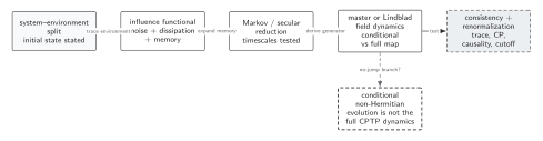
The solid path separates the exact environmental trace from the later memory and secular approximations. In field theory, the final consistency node includes the cutoff dependence of rates and Lamb shifts and the preservation of gauge or other constraints. A Redfield equation that fails the GKSL coefficient-matrix test is not made Lindbladian by notation, and the dashed no-jump evolution is not the full channel. The diagram is schematic and not to scale.

In text, compare the bath correlation time with relaxation times, retain near-degenerate Bohr-frequency blocks when required, and renormalize coherent and dissipative operators together. Then test trace preservation and complete positivity on the regulated physical state space.

Exercises

Show that the secular dissipator preserves the trace.

Solution

For each pair $\alpha,\beta$, cyclicity gives $\operatorname{Tr}(A_\beta\rho A_\alpha^\dagger)=\operatorname{Tr}(A_\alpha^\dagger A_\beta\rho)$. The anticommutator contributes the negative of the same quantity. The Hamiltonian commutator also has zero trace, so $d\operatorname{Tr}\rho/dt=0$.

Why does $\tau_E\ll\tau_S$ not by itself justify full secularization?

Solution

Short memory justifies replacing the delayed state by its present value. Secularization compares differences of system frequencies with the relaxation rate or chosen coarse-graining time. Two nearly degenerate transitions can satisfy $\tau_E\ll\tau_S$ while their relative phase remains slow, so their interference must be retained.

Continue to guarantees and memory

Lindblad field dynamics examines the CPTP semigroup and trajectory interpretation. Non-Markovian dynamics keeps the memory kernel when the Markov step fails, and consistency tests assemble independent checks for any proposed generator.

References

• Breuer, Heinz-Peter, and Francesco Petruccione. The Theory of Open Quantum Systems. Oxford: Oxford University Press, 2002. doi:10.1093/acprof:oso/9780199213900.001.0001.
• Davies, E. Brian. “Markovian Master Equations.” Communications in Mathematical Physics 39 (1974): 91–110. doi:10.1007/BF01608389.
• Gorini, Vittorio, Andrzej Kossakowski, and E. C. George Sudarshan. “Completely Positive Dynamical Semigroups of N-Level Systems.” Journal of Mathematical Physics 17 (1976): 821–825. doi:10.1063/1.522979.
• Nakajima, Sadao. “On Quantum Theory of Transport Phenomena: Steady Diffusion.” Progress of Theoretical Physics 20 (1958): 948–959. doi:10.1143/PTP.20.948.
• Rivas, Ángel, Susana F. Huelga, and Martin B. Plenio. “Quantum Non-Markovianity: Characterization, Quantification and Detection.” Reports on Progress in Physics 77 (2014): 094001. doi:10.1088/0034-4885/77/9/094001. Open preprint.
• Zwanzig, Robert. “Ensemble Method in the Theory of Irreversibility.” Journal of Chemical Physics 33 (1960): 1338–1341. doi:10.1063/1.1731409.