Thermal Self-Energies and Mass Definitions

A “thermal mass” is not a unique number. A screening mass governs static spatial decay, a pole mass solves a real-time dispersion relation, an asymptotic mass describes a hard high-momentum excitation, a curvature mass is a Hessian of a thermodynamic potential, and a quasiparticle mass is meaningful only together with its momentum dependence and width. They can agree at leading order in a simple scalar theory and differ as soon as frequency dependence, damping, gauge structure, or resummation matters.

The distinct pole, screening, and quasiparticle mass limits are developed in Le Bellac 1996, chs. 5–6.

Required background. Thermal Propagators and Spectral Representations fixes retarded and Euclidean functions. Thermal Loop Expansions and Scale Power Counting fixes kinematic regimes. Helpful background. Schwinger–Dyson Identities supplies the exact inverse-propagator relation.

Self-energy and analytic continuation

For a scalar, define the retarded propagator by

$$G_R^{-1}(\omega,\mathbf p) =(\omega+i0)^2-\mathbf p^2-m^2 -\Pi_R(\omega,\mathbf p).$$

The Euclidean inverse is

$$G_E^{-1}(i\omega_n,\mathbf p) =\omega_n^2+\mathbf p^2+m^2 +\Pi_E(i\omega_n,\mathbf p).$$

With the displayed definitions, the upper-half-plane relation $G_E(i\omega_n,\mathbf p)=-G_R(i\omega_n,\mathbf p)$ for $n>0$ implies $\Pi_E(i\omega_n,\mathbf p)=\Pi_R(i\omega_n,\mathbf p)$ on that branch. Negative Matsubara frequencies continue through the lower-half-plane, advanced branch; the zero mode is a separately specified static limit. A source that assigns the opposite sign in its Dyson definition must translate both propagator and self-energy relations together. Continuing a truncated expression must preserve its cuts and sheet; substituting $i\omega_n\to\omega+i0$ after an expansion that was valid only at $\omega_n=0$ is not legitimate.

Five mass definitions

Screening mass. The longest static spatial correlation length is obtained from the nearest pole of the zero-frequency Euclidean correlator,

$$-m_{\mathrm{scr}}^2+m^2 +\Pi_E(0,\mathbf p^2=-m_{\mathrm{scr}}^2)=0.$$

It is a spatial quantity. In gauge theory, a gauge-invariant screening channel should be defined by an eligible composite operator or matched EFT observable.

Pole mass and width. At $\mathbf p=0$, a quasiparticle pole $\omega_*=M-i\Gamma$ solves

$$\omega_*^2-m^2-\Pi_R(\omega_*,\mathbf0)=0$$

on the appropriate retarded sheet. For a narrow mode evaluated consistently,

$$M^2=m^2+\operatorname{Re}\Pi_R(M,\mathbf0), \qquad \Gamma=-\frac{\operatorname{Im}\Pi_R(M,\mathbf0)} {2M-\partial_\omega\operatorname{Re}\Pi_R(M,\mathbf0)}.$$

Dropping the derivative is an additional weak-width approximation.

Here $\Gamma$ is the pole damping rate in $\omega_*=M-i\Gamma$; the full Breit–Wigner energy width is $2\Gamma$ when that narrow-resonance description applies.

Asymptotic mass. For $p\gg$ the soft scale, write

$$\omega(p)=p+\frac{m_\infty^2}{2p}+\cdots.$$

$m_\infty$ enters hard propagation and collinear rates; it need not equal the static screening mass.

Curvature mass. For order parameter $\varphi$,

$$m_{\mathrm{curv}}^2= \left.\frac{\partial^2V_{\mathrm{eff}}}{\partial\varphi^2} \right|_{\varphi_{\min}}.$$

It is the zero-momentum Hessian in a specified field normalization and gauge. It can be gauge and scheme dependent even when a physical phase criterion is not.

Quasiparticle mass. A fitted dispersion parameter is useful only where the spectral function has an isolated narrow peak and the fit window, width, and continuum background are controlled.

Scalar leading-order agreement and later separation

In weakly coupled massless $\lambda\phi^4/4!$ theory, the one-loop tadpole is momentum independent:

$$\Pi_{\mathrm{th}}=\frac{\lambda T^2}{24}.$$

At this order, screening, zero-momentum pole, and curvature masses all receive the same shift. This agreement is accidental to a local frequency-independent self-energy. At higher order, $\Pi_R(\omega,p)$ develops momentum dependence and an imaginary part; different limits then sample different values.

Mass-definition checklist

Name	Equation/observable	Limit	Primary failure
screening	static spatial pole or exponential decay	$\omega=0$, complex $p$	confused with real-time pole
pole	zero of $G_R^{-1}$	complex $\omega$, fixed real $p$	wrong sheet or broad mode
asymptotic	hard dispersion correction	$p\gg$ soft scales	applied to static sector
curvature	effective-action Hessian	zero external momentum	gauge/field-coordinate dependence
fitted quasiparticle	spectral peak model	declared window and resolution	peak assumed rather than resolved

The chapter renormalization table separates mass reorganization from ultraviolet counterterms.

The schematic below organizes the relationships used on this page. Inspect it with this question in mind: How does a thermal loop calculation pass from scale counting to a physical observable?

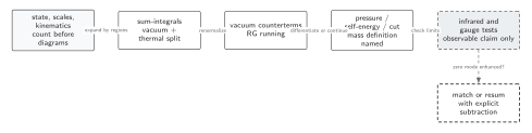
Thermal power counting chooses hard and soft regions; sum-integrals are split into vacuum and thermal parts, vacuum counterterms renormalize them, and mass, width, infrared, RG, and gauge checks bound the final observable. Solid connections show the primary relation; dashed outlines or arrows mark qualifications and failure boundaries. The diagram is schematic and not to scale.

The surrounding discussion supplies the relevant equations and checks in text form; the figure is a navigational summary.

Exercise

Let $\Pi_R(\omega,p)=aT^2+b\omega^2+cp^2$ with small $a,b,c$. Find the leading screening and zero-momentum pole masses for $m=0$.

Solution

The static Euclidean continuation gives $m_{\mathrm{scr}}^2\simeq aT^2/(1+c)$ in the displayed sign convention. The pole equation gives $M^2(1-b)=aT^2$, so $M^2\simeq aT^2/(1-b)$. Momentum and frequency dependence separate the two even without a width.

References

• Le Bellac, Michel. Thermal Field Theory. Cambridge: Cambridge University Press, 1996. doi:10.1017/CBO9780511721700.
• Pisarski, Robert D. “Scattering Amplitudes in Hot Gauge Theories.” Physical Review Letters 63, no. 11 (1989): 1129–1132. doi:10.1103/PhysRevLett.63.1129.