The Hydrodynamic Limit and Slow Variables

Hydrodynamics applies when a disturbance evolves on scales much longer than microscopic relaxation scales because conservation laws or another declared mechanism prevent its rapid decay. The hydrodynamic limit is therefore a joint limit in frequency, wave number, and any small symmetry-breaking rate—not a synonym for “locally thermal” and not a fixed list of fluid variables.

Required background. Spurions, Local Counterterms, and Symmetry Response supplies the source-response Ward identities from which conserved-density poles follow.

Helpful background. Linearized Kinetics and Relaxation Modes shows the microscopic separation between collision zero modes and gapped modes. Memory Functions and Slow-Mode Projection develops the complementary projection formalism.

Conservation produces a soft pole

Consider a conserved scalar density $n$ and current $\mathbf j$,

$$\partial_t n+\boldsymbol\nabla\!\cdot\!\mathbf j=0.$$

If all nonconserved local variables relax in a time $\tau_{\mathrm{micro}}$, locality and rotational invariance permit the constitutive expansion

$$\mathbf j=-D\boldsymbol\nabla n+O(\partial^2,n^2).$$

For $e^{-i\omega t+i\mathbf k\cdot\mathbf x}$, conservation closes to

$$-i\omega+Dk^2+O(k^4)=0, \qquad \omega(k)=-iDk^2+O(k^4).$$

The rate vanishes as $k\to0$ because a spatially uniform conserved excess cannot decay. A retarded density correlator consequently has the low-energy form

$$G^R_{nn}(\omega,k) = -\chi\,\frac{Dk^2}{-i\omega+Dk^2} +\text{terms analytic near }(0,0),$$

where $\chi$ is the static susceptibility. This uses the site convention $G^R=-i\theta(t)\langle[n(t),n(0)]\rangle$: for a Hamiltonian source $H\to H-\int\mu n$, the physical response is $-G^R$ and $G^R(0,k\to0)=-\chi$. Kadanoff and Martin derive this connection between local conservation, constitutive closure, and hydrodynamic singularities Kadanoff and Martin 1963, §§2–3, pp. 421–430.

Energy and longitudinal momentum instead form a reversible pair. Conservation gives a matrix linear in $k$, producing $\omega=\pm c_s k+O(k^2)$ rather than diffusion. The mechanism is the same: exact conservation forces eigenvalues to approach zero, while reversible couplings determine whether the approach is linear or quadratic in $k$.

Scale separation defines the expansion

Let $\tau_{\mathrm{micro}}$ and $\ell_{\mathrm{micro}}$ characterize the least-damped omitted mode and the shortest length resolved by a local constitutive law. Ordinary hydrodynamics requires

$$|\omega|\tau_{\mathrm{micro}}\ll1, \qquad k\ell_{\mathrm{micro}}\ll1.$$

These inequalities concern derivatives, not amplitudes. Nonlinear hydrodynamics can describe order-one changes spread over long distances; linear response imposes a separate small-amplitude approximation. Fluctuating hydrodynamics adds a loop or noise expansion, and near criticality that expansion can fail even while $k\ell_{\mathrm{micro}}$ is small.

The constitutive relation integrates out modes with nonzero relaxation rates at $k=0$. If the smallest omitted rate is not well separated from the target frequency, the resulting kernels become strongly frequency dependent and a local derivative expansion ceases to be economical. Kovtun gives this pole-based formulation and its charged and stress-tensor examples Kovtun 2012, §2, pp. 19–29, Open PDF.

Approximately conserved variables

Suppose a density obeys

$$\partial_t n+\boldsymbol\nabla\!\cdot\!\mathbf j=-\Gamma n, \qquad \Gamma\tau_{\mathrm{micro}}\ll1.$$

Then

$$\omega=-i\Gamma-iDk^2+\cdots .$$

This mode is not hydrodynamic in the strict $k\to0$ sense because its gap is nonzero. It is nevertheless quasihydrodynamic on times $t\ll\Gamma^{-1}$ or whenever $\Gamma$ is part of the controlled small-parameter counting. Integrating it out at $\omega\sim\Gamma$ produces a memory kernel; retaining it restores a local enlarged system.

The same decision arises for a weakly broken symmetry, a critical order parameter with critical slowing down, spin density with a long relaxation time, axial charge with a small violation rate, or a nonhydrodynamic stress mode promoted in a transient theory. The page Hydro+ and Parametrically Slow Critical Modes treats the critical example; the present criterion is the universal selection rule.

Completeness is a physical hypothesis

A charged normal fluid away from criticality usually retains energy density, momentum density, and each independent conserved charge density. This set is incomplete when:

• a continuous symmetry is spontaneously broken, requiring a Goldstone phase;
• a critical mode relaxes on the hydrodynamic time scale;
• integrability supplies infinitely many relevant conservation laws;
• a background field changes which momentum components are conserved;
• an external drive removes energy conservation or creates a new slow phase;
• an initial state supports a parametrically narrow quasiparticle or coherent mode.

No pole calculation can repair an omitted variable. A fit may hide the omission in a frequency-dependent “transport coefficient,” but that coefficient is then not the local constitutive datum it was assumed to be.

Checks and limitations

Three checks catch most mistakes. First, at $k=0$ every exactly conserved density must have zero relaxation rate. Second, residues must obey the relevant Ward identity and static susceptibility. Third, adding a small breaking rate must move the pole continuously from $-iDk^2$ to $-i\Gamma-iDk^2$, not remove it discontinuously.

The hydrodynamic pole is an infrared statement. Extending $-iDk^2$ to arbitrarily large $k$ gives a parabolic PDE with instantaneous tails, but microscopic causality is not decided by extrapolating a truncated low-$k$ series. Whether a chosen macroscopic formulation itself has a causal well-posed initial-value problem is the separate subject of Strong Hyperbolicity, Stability, and Causal Propagation.

The first two boxes in the schematic isolate this page’s central step: conservation selects slow densities, while coarse graining is the additional physical assumption that permits a local-equilibrium description. Follow the remaining boxes only as a preview of the closures that later pages will test.

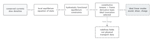
Conservation provides the parametrically slow densities but does not by itself prove local equilibration. The later source, constitutive, and mode stages require the scale separation and completeness hypotheses stated on this page. The diagram is a qualitative dependency map, not a plot of relaxation times or a claim that every conserved density is sufficient for closure.

In text: identify all exact and approximate conservation laws; verify a gap to omitted modes; assume local equilibration only inside the resulting frequency and wavelength window; then construct and test a constitutive closure. If another mode becomes parametrically slow, it must be added before the later stages in the diagram are valid.

Exercise

A nearly conserved charge has constitutive current $\mathbf j=-D\nabla n$ and relaxation rate $\Gamma$. Couple a source $\mu$ so that the equilibrium response is $\delta n=\chi\mu$. Find a retarded correlator with the correct static limit.

Solution

The sourced relaxation equation can be written

$$(\partial_t+\Gamma-D\nabla^2)\delta n = (\Gamma-D\nabla^2)\chi\mu.$$

Therefore

$$G^R_{nn}(\omega,k) = -\chi\, \frac{\Gamma+Dk^2}{-i\omega+\Gamma+Dk^2}.$$

At $\omega=0$ it equals $-\chi$, so the response $-G^R$ equals $\chi$; at vanishing source its pole is $\omega=-i(\Gamma+Dk^2)$. Contact-term conventions can redistribute analytic pieces, but not this pole and its static normalization.

Where this leads

Conservation Laws and Hydrodynamic Fields now turns the slow densities into covariant stress and current variables. Generalized Hydrodynamics of Integrable Systems treats the distinct case in which the conserved set is extensive or infinite.

References

• Kadanoff, Leo P., and Paul C. Martin. 1963. “Hydrodynamic Equations and Correlation Functions.” Annals of Physics 24: 419–469. DOI.

• Kovtun, Pavel. 2012. “Lectures on Hydrodynamic Fluctuations in Relativistic Theories.” Journal of Physics A: Mathematical and Theoretical 45: 473001. DOI. Open PDF.