Dynamic Scaling and Critical Slowing Down

Near a continuous transition, the equilibrium correlation length diverges and the longest relaxation time scales as $\tau_{\mathrm{rel}}\sim\xi^z$. The dynamic exponent $z$ depends on the slow-variable dynamics, not only on the static fixed point. For a finite-rate ramp, evolution freezes out when the relaxation time becomes comparable to the time remaining to the critical point.

Required background. Use critical exponents and hyperscaling and correlations, susceptibilities, and correlation lengths.

Helpful background. Dynamic universality classes determine which $z$ should be used.

Dynamic scaling

Let the reduced control parameter be $\epsilon=(g-g_c)/g_c$. In the scaling regime,

$$\xi=\xi_0|\epsilon|^{-\nu}, \qquad \tau_{\mathrm{rel}}=\tau_0\left(\frac{\xi}{\xi_0}\right)^z =\tau_0|\epsilon|^{-\nu z}.$$

A two-point dynamic structure factor has the scaling form

$$S(k,\omega;\epsilon) =k^{-2+\eta-z}\, \Phi\!\left(\frac{\omega}{k^z},k\xi\right),$$

up to operator normalization and additional scaling fields. This form assumes one dominant relaxation scale. Propagating and diffusive modes, multiple conserved fields, or dangerously irrelevant variables can require several frequency variables or crossover exponents.

Critical slowing down means local equilibration fails first at the largest wavelengths. Finite size cuts off $\xi$ at $L$, giving $\tau_L\sim L^z$. A measured saturation can therefore be a box effect rather than a microscopic relaxation time.

The last box of the schematic is a testable scaling claim, not an automatic consequence of writing a Langevin equation. The dynamic exponent and scaling function depend on the complete set of slow variables, conservation laws, and reversible couplings.

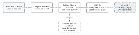
Dynamic scaling follows only after the stochastic process and its slow-variable content have been specified and the corresponding response theory has a controlled scaling regime. Detailed balance is optional and must be checked; nonequilibrium fixed points can have different scaling. Kibble–Zurek freeze-out further requires a declared ramp and a comparison between relaxation and driving timescales. The diagram is schematic and not to scale.

The sections Dynamic scaling, Kibble–Zurek freeze-out, and Failure tests provide the text and equation equivalent of the scaling endpoint and its assumptions.

Kibble–Zurek freeze-out

For a linear ramp $\epsilon(t)=t/\tau_Q$ through $t=0$, the freeze-out argument of Zurek 1985 compares

$$\tau_{\mathrm{rel}}(\epsilon) \quad\text{with}\quad \left|\frac{\epsilon}{\dot\epsilon}\right|=|t|.$$

The freeze-out condition gives

$$|\hat\epsilon| =\left(\frac{\tau_0}{\tau_Q}\right)^{1/(1+\nu z)}, \qquad \hat\xi =\xi_0\left(\frac{\tau_Q}{\tau_0}\right)^{\nu/(1+\nu z)},$$

and

$$\hat t =\tau_0^{1/(1+\nu z)} \tau_Q^{\nu z/(1+\nu z)}.$$

These are scaling estimates, not exact switching times. The adiabatic–impulse picture compresses a smooth crossover, and amplitudes depend on the ramp, initial state, and operational definition.

For defects of codimension $c$ whose initial separation is controlled by $\hat\xi$, one often estimates $n_{\mathrm{def}}\sim\hat\xi^{-c}$. Defect annihilation after crossing, inhomogeneous fronts, topology, gauge fields, and finite detection time can change the observed exponent.

Checked mean-field Model-A example

For a Gaussian nonconserved order parameter, $\nu=1/2$ and the relaxation rate is $\Gamma(k^2+\xi^{-2})$, so $z=2$. The formulas give

$$\hat\xi\propto\tau_Q^{1/4}, \qquad \hat t\propto\tau_Q^{1/2}.$$

Directly, at $k=0$ the relaxation time is proportional to $|\epsilon|^{-1}$; equating $\tau_0/|\epsilon|$ with $\tau_Q|\epsilon|$ gives $|\hat\epsilon|\sim(\tau_0/\tau_Q)^{1/2}$ and the same $\hat\xi$ scaling.

Failure tests

• Demonstrate the static and dynamic scaling windows separately.
• Identify all conserved and reversible slow modes before assigning $z$.
• Repeat at several sizes and ramp shapes.
• Vary the initial distance from criticality and initial correlations.
• Test for crossover between multiple dynamic exponents.
• Separate freeze-out scaling from post-crossing coarsening and defect annihilation.

Exercise

For a power-law ramp $\epsilon(t)=\operatorname{sgn}(t)|t/\tau_Q|^r$, derive the scaling of $|\hat\epsilon|$.

Solution

$|\epsilon/\dot\epsilon|=|t|/r$. With $|t|=\tau_Q|\epsilon|^{1/r}$, the condition $\tau_0|\epsilon|^{-\nu z}=\tau_Q|\epsilon|^{1/r}/r$ gives $|\hat\epsilon|\sim(r\tau_0/\tau_Q)^{r/(1+r\nu z)}$.

Continue

Classify the slow variables on dynamic universality classes and distinguish freeze-out from later coarsening and aging.

References

• Kibble, T. W. B. (1976). “Topology of Cosmic Domains and Strings.” Journal of Physics A 9, 1387–1398. DOI.
• Zurek, W. H. (1985). “Cosmological Experiments in Superfluid Helium?” Nature 317, 505–508. DOI.