From Kadanoff–Baym to Kinetic Theory

A Boltzmann equation follows from Kadanoff–Baym evolution only after several independent reductions: Wigner gradients are truncated, spectral weight is projected onto separated quasiparticle shells, memory and initial-correlation terms are localized, higher correlations are factorized, and the self-energy is evaluated in a closure consistent with conservation. Each step can fail while the others remain valid.

Required background. Use the Wigner and gradient expansion and spectral/statistical evolution.

Helpful background. Quasiparticle shell and gradient counting tests the resulting hierarchy quantitatively.

Unreduced transport equation

At first Wigner-gradient order, the transport/constraint separation derived in Botermans and Malfliet 1990, §§ 3–4 has the schematic form

$$\{\mathcal H,F\}_{\mathrm{PB}} =\Sigma_\rho F-\Sigma_F\rho+\mathcal B_{\mathrm{backflow}} +O(\partial_X^2),$$

where $\mathcal H=p^2-m^2-\operatorname{Re}\Sigma_R$, $\rho$ is the spectral function, and $\mathcal B_{\mathrm{backflow}}$ contains first-order derivatives of self-energies and propagators. The companion constraint equation determines spectral support. A kinetic equation is not obtained by discarding the constraint.

The quasiparticle ansatz writes

$$F(X,p)=-i\left(\frac12+f(X,p)\right)\rho(X,p)$$

for bosons and approximates

$$\rho(X,p)\longrightarrow 2\pi i\,\operatorname{sgn}(p^0)\, \delta[\mathcal H(X,p)] .$$

Integrating over positive-frequency support produces a distribution $f(X,\mathbf p)$. This requires a narrow peak, a unique branch, and test functions smooth across its width. It fails for broad continua, overlapping branches, thresholds, or coherent matrices.

The reduction steps

1. Gradient expansion. Center-coordinate variation must be slow relative to the support of relative-time and memory kernels. Keep all terms at one declared order, including backflow and mean-field forces.
2. Shell projection. Solve the spectral constraint and integrate over $p^0$. The width-to-energy ratio and separation from other shells must be small.
3. Closure. Express $\Sigma_F$ and $\Sigma_\rho$ in terms of the retained distributions using a controlled loop, coupling, $1/N$, or effective-theory expansion.
4. Molecular chaos. Factorize incoming multiparticle correlations at the collision scale. Initial and dynamically generated correlations omitted here are the source of kinetic irreversibility.
5. Markov limit. Extend or localize memory integrals only after showing their correlation time is short compared with the evolution of $f$. Energy-conserving delta functions emerge from a long-time limit; at finite time they are broadened.
6. Vertex and soft resummation. Include screening, widths, collinear interference, or ladder corrections at the same parametric order as the nominal scattering graph.

The resulting equation has the form

$$p^\mu\partial_\mu f+\mathcal F^\mu\partial_{p^\mu}f=C[f],$$

but its $C[f]$ inherits every choice above.

The diagram is a compact checklist for the reduction just performed. No single arrow is automatic: shell projection, gradient truncation, memory loss, collision construction, and scalarization each require their own small parameter or convergence test.

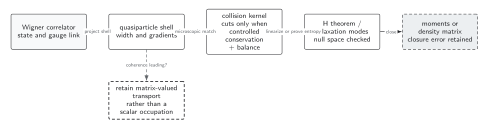
Kinetic theory follows from the two-time equations only after a controlled Wigner and gradient expansion, spectral or quasiparticle projection, and a justified treatment of memory. Weak-coupling cuts can then produce a gain–loss kernel, but conservation, detailed balance, and any entropy theorem must still be verified. If coherence is leading, the scalar route is replaced by the dashed matrix-valued branch. The diagram is schematic and not to scale.

The sections Unreduced transport equation, The reduction steps, and What creates irreversibility give the text and equation equivalent of the first four boxes and their assumptions.

Checked scalar 2↔2 limit

For weak $\lambda\phi^4$ theory with narrow massive quasiparticles, the setting-sun self-energy yields a $2\leftrightarrow2$ collision term after shell projection and the long-time limit:

$$C_1\propto\int d\Pi_2d\Pi_3d\Pi_4\, (2\pi)^4\delta^4(p_1+p_2-p_3-p_4)|\mathcal M|^2 \left[f_3f_4(1+f_1)(1+f_2) -f_1f_2(1+f_3)(1+f_4)\right].$$

The two terms are gain and loss, and Bose factors follow from Wightman components. The energy delta function is the Markov/long-time limit of an oscillatory memory integral. At finite duration or finite width, replacing that integral by an exact delta function can overstate kinematic suppression near threshold.

Integrating $C_1$ with $p_1^\mu$ and summing the four relabeled legs gives zero because the delta function enforces $p_1+p_2-p_3-p_4=0$. This conservation proof works only if the numerical quadrature and all crossed contributions use identical normalization.

What creates irreversibility

The parent closed quantum evolution is time-reversal invariant. Monotonic kinetic entropy arises after discarded correlations are replaced by factorized functions and memory is localized with retarded boundary conditions. Recurrences and phase information are removed from the effective state description. This is controlled coarse graining, not microscopic nonunitarity.

Failure tests

• Compare first- and second-gradient terms on the actual solution.
• Vary the spectral width and shell projection; check thresholds and branch overlap.
• Restore a finite memory window and initial correlations once.
• Derive the collision kernel from the same self-energy closure used in the spectral equation.
• Test collision invariants and detailed balance analytically and numerically.
• Compare the reduced solution with the parent two-time calculation over the claimed regime; a calculation can execute that comparison later, but no calculation result is assumed here.

Exercise

For an oscillatory memory integral $\int_0^t ds\,e^{i\Delta E s}$, show how energy conservation emerges as $t\to\infty$.

Solution

The integral is $e^{i\Delta E t/2}\,2\sin(\Delta E t/2)/\Delta E$. Its squared magnitude divided by $t$ approaches $2\pi\delta(\Delta E)$ distributionally. At finite $t$, the peak has width of order $1/t$, so exact energy conservation is a long-time approximation rather than a pointwise identity of the finite-memory kernel.

Continue

Quantify shell and gradient control on quasiparticle power counting and implement the licensed processes on collision kernels.

References

• Botermans, W., and Malfliet, R. (1990). “Quantum Transport Theory of Nuclear Matter.” Physics Reports 198, 115–194. DOI.
• Danielewicz, P. (1984). “Quantum Theory of Nonequilibrium Processes, I.” Annals of Physics 152, 239–304. DOI.
• Kadanoff, L. P., and Baym, G. (1962). Quantum Statistical Mechanics. New York: W. A. Benjamin. Internet Archive record.