Local Equilibrium and Hydrostatic Constraints

Local equilibrium is a controlled parametrization of a slowly varying state by a thermal vector and chemical twist. Hydrostatics is narrower: it describes configurations invariant under a timelike symmetry of the background sources. A hydrostatic generating functional fixes equilibrium and nondissipative constitutive data, but it cannot determine generic dissipative evolution away from stationarity.

Required background. Conservation Laws and Hydrodynamic Fields fixes the source-covariant stress and current conventions. Thermal Density Operators and the KMS Condition supplies the equilibrium density-operator structure.

Helpful background. Coupling to Background Gauge Fields and Bundles explains background gauge covariance and its global qualifications.

Local Gibbs data

On a spacelike hypersurface $\Sigma$, introduce

$$\beta^\mu(x)=\frac{u^\mu(x)}{T(x)}, \qquad \nu(x)=\frac{\mu(x)}{T(x)}.$$

A local Gibbs operator has the schematic form

$$\rho_{\mathrm{LE}} = \frac{1}{Z_{\mathrm{LE}}} \exp\!\left[ -\int_\Sigma \mathrm d\Sigma_\mu \left( \beta_\nu T^{\mu\nu}-\nu J^\mu \right) \right].$$

For constant $\beta^\mu=(1/T,\mathbf0)$ and $\nu=\mu/T$, the exponent is $-(H-\mu Q)/T$. Away from global equilibrium, $\rho_{\mathrm{LE}}$ is a matching ansatz at the chosen time, not a stationary density operator. Its hypersurface dependence is controlled only when gradients are small and the constitutive evolution is supplied.

The gauge-covariant datum is not $\nu$ alone. Under $A_\mu\mapsto A_\mu+\partial_\mu\alpha$, the thermal transformation includes a compensating scalar $\Lambda_\beta$; one may use the invariant combination

$$\widehat\mu = T\left(\Lambda_\beta+\beta^\mu A_\mu\right).$$

Different sign conventions for $\Lambda_\beta$ are common. The invariant combination and the grand-canonical exponent, not the symbol, are the translation checks.

Hydrostatic stationarity

A configuration is hydrostatic when the sources admit a timelike thermal symmetry:

$$\mathcal L_\beta g_{\mu\nu}=0, \qquad \mathcal L_\beta A_\mu+\partial_\mu\Lambda_\beta=0.$$

The first equation says that $\beta^\mu$ is a Killing vector. It includes Tolman–Ehrenfest redshift: the locally measured temperature can vary in a gravitational field even though the state is globally stationary. The second says that the gauge field is invariant up to a gauge transformation.

These are stronger conditions than “gradients are small.” A shear flow can vary slowly but fail to be hydrostatic; an equilibrium rotating state can have nonzero vorticity while satisfying a Killing condition. Banerjee et al. construct the stationary partition function and show how it constrains relativistic constitutive relations order by order Banerjee et al. 2012, §§2–3, pp. 5–17, Open PDF.

Generating functional and ideal response

For stationary sources, let $W_{\mathrm{hs}}[g,A]=\log Z_{\mathrm{hs}}$. Its variations define equilibrium one-point functions,

$$\delta W_{\mathrm{hs}} = \frac12\int \mathrm d^d x\,\sqrt{-g}\, T_{\mathrm{hs}}^{\mu\nu}\delta g_{\mu\nu} +\int \mathrm d^d x\,\sqrt{-g}\, J_{\mathrm{hs}}^\mu\delta A_\mu .$$

At zeroth derivative order the only scalar input is the pressure:

$$W_{\mathrm{hs}}^{(0)} = \int_{\Sigma_{\mathrm{stat}}} \mathrm d^{d-1}x\,\sqrt{\gamma}\, \frac{p(T,\mu)}{T}.$$

Varying $T$ and $\mu$ through the stationary sources and using

$$\mathrm dp=s\,\mathrm dT+n\,\mathrm d\mu, \qquad \epsilon+p=Ts+\mu n,$$

gives

$$T_{\mathrm{hs}}^{\mu\nu} =\epsilon u^\mu u^\nu+pP^{\mu\nu}, \qquad J_{\mathrm{hs}}^\mu=n\,u^\mu .$$

Thus the perfect-fluid form is a response statement, not merely an appeal to isotropy. Jensen et al. show that the same equilibrium functional organizes nondissipative transport without assuming a particular entropy-current representative Jensen et al. 2012, pp. 1–4.

Magnetization and polarization currents

Derivative terms in $W_{\mathrm{hs}}$ can depend on $F_{\mu\nu}$, curvature, vorticity, and scalar gradients. Their variations include currents of the form

$$J^\mu_{\mathrm{mag}}=\nabla_\nu M^{\nu\mu}, \qquad M^{\nu\mu}=-M^{\mu\nu}.$$

They are identically conserved in the smooth bulk: antisymmetry and the symmetry of the Ricci tensor give $\nabla_\mu\nabla_\nu M^{\nu\mu}=0$. Topology and boundaries still affect the integrated current. Such currents circulate in equilibrium and can contribute to local response, yet they are not through-sample transport currents. Kubo formulae must subtract the appropriate magnetization terms; otherwise an equilibrium circulation is misidentified as conductivity.

Boundaries make this distinction physical rather than disposable: a bulk magnetization current can be accompanied by an edge current. The generating functional must therefore record boundary conditions and any boundary counterterms.

What hydrostatics cannot fix

Shear viscosity, bulk viscosity, and ordinary longitudinal conductivity multiply structures that vanish in exact hydrostatics. No variation of a stationary Euclidean functional determines their real-time dissipative values. Hydrostatics can constrain nondissipative coefficients and relations among equilibrium responses; entropy production, retarded boundary conditions, and Schwinger–Keldysh/KMS structure supply additional dynamical information.

An anomaly can add hydrostatic terms with quantized or matching-controlled coefficients, but it does not license replacing dynamical anomalous transport by an equilibrium formula outside its regime. Likewise, a local Gibbs ansatz does not prove rapid local equilibration.

The middle of the schematic summarizes the controlled reach of hydrostatics. Inspect the passage from local equilibrium to a source-dependent hydrostatic functional, and then note that constitutive dynamics still require an expansion and a frame choice.

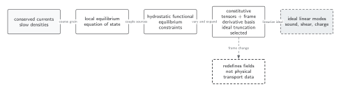
Stationary sources and the thermal Killing data determine equilibrium response and constrain hydrostatic constitutive terms. They do not determine dissipative coefficients, noise, or evolution away from hydrostatic equilibrium. The diagram is a schematic dependency map; neither horizontal distance nor box style represents an expansion parameter or evidence level.

In text: construct the local Gibbs data $(\beta^\mu,\Lambda_\beta)$, impose source-compatible stationarity, vary the hydrostatic functional to obtain equilibrium stress and current, and separate magnetization circulation from bulk transport. Dissipative completion begins only after that equilibrium information has been matched.

Exercise

Show that rigid rotation in flat spacetime can be hydrostatic. Take $\beta=\beta_0(\partial_t+\Omega\partial_\phi)$ in cylindrical coordinates.

Solution

Both $\partial_t$ and $\partial_\phi$ are Killing vectors, so their constant linear combination obeys $\mathcal L_\beta g=0$. Its norm is

$$\beta^2=\beta_0^2(1-\Omega^2r^2),$$

hence

$$T(r)=\frac{1}{\sqrt{\beta^2}} = \frac{T_0}{\sqrt{1-\Omega^2r^2}}.$$

The state is meaningful only inside the light cylinder $r<|\Omega|^{-1}$, where $\beta$ remains timelike. Nonzero vorticity is therefore compatible with hydrostatics; loss of a timelike thermal vector is the limiting obstruction.

Where this leads

Hydrodynamic Frames and Constitutive Data explains why the fields extracted from a nonstationary configuration are not unique. The later page Contact Terms, Magnetization Currents, and Order of Limits carries the equilibrium-current distinction into transport extraction.

References

• Banerjee, Nabamita, et al. 2012. “Constraints on Fluid Dynamics from Equilibrium Partition Functions.” Journal of High Energy Physics 2012 (9): 046. DOI. Open PDF.

• Jensen, Kristan, Matthias Kaminski, Pavel Kovtun, René Meyer, Adam Ritz, and Amos Yarom. 2012. “Towards Hydrodynamics without an Entropy Current.” Physical Review Letters 109: 101601. DOI. Open PDF.