Thermal Modes, Matching, and EFT Power Counting

A thermal effective field theory is defined by what it predicts, not merely by deleting high-frequency fields. One first chooses an observable and its external kinematics, separates the modes that can affect it, integrates out the remaining modes, and fixes the resulting coefficients by matching. The calculation is controlled only when its scale hierarchy, operator truncation, overlap subtraction, and first omitted term are all explicit.

The mode-matching construction for high-temperature thermodynamics is demonstrated by Braaten and Nieto 1995, §§ II–III, pp. 6992–6999.

Required background. Thermal Loop Expansions and Scale Power Counting supplies thermal scale counting. Scale Separation, Locality, and the Domain of an EFT supplies the locality criterion for integrating out modes. Helpful background. Modes, Virtualities, and EFT Scale Separation develops the general regions language.

Match an observable, not a slogan

Let a full theory contain a hard scale $M$ and a retained scale $Q\ll M$. For external momenta of order $Q$, its effect is represented by

$$S_{\mathrm{EFT}}[\phi_<] =\int \mathrm d^d x\,\sum_i C_i(M,\mu_f)\,\mathcal O_i(\phi_<;\mu_f),$$

where $\mu_f$ separates the matched and retained regions. The coefficients $C_i$ are fixed by requiring a chosen set of full-theory and EFT correlators, amplitudes, or thermodynamic derivatives to agree through a declared order. A valid basis contains every operator allowed by the retained symmetries at that order, including operators removable only after a stated field redefinition.

At finite temperature, “hard” and “soft” are observable-dependent. Useful labels include

• nonzero bosonic Matsubara modes, with gaps at least $2\pi T$;
• fermionic Matsubara modes, with gaps at least $\pi T$;
• bosonic zero modes, which can remain soft and effectively three-dimensional;
• quasiparticle poles, widths, cuts, and collective modes in real time; and
• dynamically generated electric, scalar, magnetic, or critical scales.

A mode may be integrated out for a static correlator but indispensable for a lightlike rate. The state, external frequency, momentum, and desired error therefore belong in the EFT definition.

Scalar dimensional reduction as a matching example

Consider Euclidean $\lambda\phi^4/4!$ theory at weak coupling. For static external momenta $p\ll2\pi T$, integrate out all nonzero Matsubara modes and define the canonically normalized zero-mode field

$$\varphi(\mathbf x)=\sqrt{\beta}\,\phi_0(\mathbf x).$$

The reduced action begins

$$S_3=\int\mathrm d^3x\left[ \frac12(\boldsymbol\nabla\varphi)^2 +\frac12m_3^2\varphi^2 +\frac{\lambda_3}{4!}\varphi^4 +\sum_{n>4}c_n\mathcal O_n \right].$$

At leading order in this convention,

$$\lambda_3=\lambda T, \qquad m_3^2=m^2+\frac{\lambda T^2}{24}+\cdots.$$

These relations are not a substitute for matching: beyond leading order, the coefficients depend on the renormalization and factorization conventions, while a physical static correlator does not. One practical match is the small-momentum inverse two-point function. Compute it in the full theory, subtract the zero-mode contribution reproduced by the EFT, and choose $m_3^2$ and derivative operators so the remainder agrees order by order.

Power counting and factorization-scale cancellation

If $Q/M=\epsilon\ll1$, an operator of dimension $d+n$ is normally suppressed by $\epsilon^n$, but thermal occupation factors and infrared propagators can change that estimate. In the scalar zero-mode sector, for example,

$$\lambda_3\int\frac{\mathrm d^3k}{(2\pi)^3} \frac1{(k^2+m_3^2)^2} \sim \frac{\lambda T}{m_3}.$$

Near a critical point $m_3\to0$, the nominal weak-coupling expansion therefore fails. The correct small parameter must be derived inside each retained region rather than inherited from the microscopic Lagrangian.

The artificial scale $\mu_f$ provides an essential check. Schematically,

$$X=X_{\mathrm{hard}}(\mu_f)+X_{\mathrm{soft}}(\mu_f) +O(\epsilon^{N+1}), \qquad \frac{\mathrm dX}{\mathrm d\ln\mu_f}=O(\epsilon^{N+1}).$$

Residual variation much larger than the first omitted order signals a missing operator, inconsistent truncation, or an unremoved overlap. Small variation is a necessary stability check, not proof that the true error is small.

Matching and double-counting table

This table is the minimum record needed to interpret a thermal EFT or reorganization. Later pages refer back to it when a method changes.

Description	Retained modes	Matched-out modes	Matching target	Required subtraction	Principal dependence	Failure test
static scalar reduction	bosonic zero mode at $p\ll2\pi T$	nonzero Matsubara modes and fermions	static one- and two-particle-irreducible correlators	zero-mode graphs reproduced in the reduced theory	renormalization and factorization scales	higher operators or $\lambda_3/m_3$ are unsuppressed
ring improvement	screened static bosonic propagator	hard self-energy insertions	soft determinant or static free energy	subtract insertions already present at fixed order	thermal-mass prescription and truncation order	result changes at the claimed order under an equivalent organization
screened or variational series	chosen massive or HTL-like free theory	compensating interaction treated perturbatively	pressure or declared correlator	add–subtract counterterm at the same order	auxiliary parameter and optimization branch	no stable solution or no improvement against a benchmark
real-time influence EFT	chosen slow $r/a$ fields	fast environmental or microscopic modes	retarded and symmetric correlators	slow-region contribution reproduced by the EFT	coarse-graining scale, contour convention, memory expansion	acausality, negative noise, or nonanalytic low-frequency kernel
gauge-plasma EFT	scale-specific electric, magnetic, or quasiparticle modes	harder gauge-covariant fluctuations	gauge-invariant static or causal observable	overlap between adjacent scale descriptions	gauge fixing internally, factorization scale	Ward identities, scale cancellation, or hierarchy fail

The table records a method’s claim ceiling. A coefficient without its target observable and subtraction cannot be transported safely to another calculation.

The schematic below organizes the relationships used on this page. Inspect it with this question in mind: How do static and real-time thermal EFTs partition hard, soft, electric, magnetic, and dissipative modes?

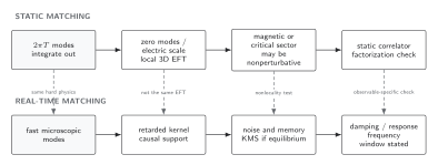
Static reduction integrates frequency-gapped modes into local Euclidean coefficients, while real-time matching fixes retarded, noise, and memory kernels; electric and magnetic sectors can require different retained theories. Solid connections show the primary relation; dashed outlines or arrows mark qualifications and failure boundaries. The diagram is schematic and not to scale.

The surrounding discussion supplies the relevant equations and checks in text form; the figure is a navigational summary.

Exercises

For the scalar example, show that $\varphi=\sqrt\beta\,\phi_0$ gives a canonical three-dimensional kinetic term and derive $\lambda_3=\lambda T$.

Solution

For a time-independent zero mode, the Euclidean integral contributes a factor $\beta$. Substituting $\phi_0=\varphi/\sqrt\beta$ gives $\beta(\boldsymbol\nabla\phi_0)^2/2=(\boldsymbol\nabla\varphi)^2/2$. The quartic term becomes $\beta\lambda\phi_0^4/4!=\lambda T\varphi^4/4!$, since $\beta^{-1}=T$.

References

• Appelquist, Thomas, and Robert D. Pisarski. “High-Temperature Yang–Mills Theories and Three-Dimensional Quantum Chromodynamics.” Physical Review D 23, no. 10 (1981): 2305–2317. doi:10.1103/PhysRevD.23.2305.
• Braaten, Eric, and Agustín Nieto. “Effective Field Theory Approach to High Temperature Thermodynamics.” Physical Review D 51, no. 12 (1995): 6990–7006. doi:10.1103/PhysRevD.51.6990.
• Ginsparg, Paul. “First- and Second-Order Phase Transitions in Gauge Theories at Finite Temperature.” Nuclear Physics B 170 (1980): 388–408. doi:10.1016/0550-3213(80)90418-6.
• Laine, Mikko, and Aleksi Vuorinen. Basics of Thermal Field Theory: A Tutorial on Perturbative Computations. Lecture Notes in Physics 925. Cham: Springer, 2016. doi:10.1007/978-3-319-31933-9.