Hydrodynamic Attractors and Asymptotic Gradient Expansions

A hydrodynamic attractor is a model- and observable-specific slow curve, or more generally a low-dimensional manifold, toward which a family of nonequilibrium solutions converges before the ordinary gradient series is accurate term by term. Its relation to asymptotics is precise in solvable transient models: factorial large-order growth and Borel singularities encode exponentially decaying nonhydrodynamic sectors. This does not make the attractor universal, nor does approaching it establish isotropy, local thermal equilibrium, or microscopic thermalization.

Required background. Strong Hyperbolicity, Stability, and Causal Propagation separates transient damping from nonlinear PDE claims. Relativistic Dissipative Hydrodynamics supplies the hydrodynamic and nonhydrodynamic mode content.

Helpful background. Hydrodynamization: the Kinetic-to-Hydrodynamic Map develops the corresponding kinetic-theory evidence and matching problem.

What an attractor statement must specify

Take boost-invariant, transversely homogeneous expansion. Proper time $\tau$ is the only spacetime variable, and the stress tensor in the local rest frame has energy density $\epsilon$, longitudinal pressure $P_L$, and transverse pressure $P_T$. A useful observable is the pressure anisotropy

$$\mathcal A(\tau) = \frac{P_T(\tau)-P_L(\tau)}{P_{\mathrm{eq}}(\epsilon(\tau))}.$$

Because it is built from stress-tensor eigenvalues, $\mathcal A$ is independent of a perturbative choice of hydrodynamic frame. A dimensionless clock such as

$$w=\tau T(\tau)$$

compares expansion time with a microscopic relaxation scale in a conformal theory. Other normalizations are legitimate, but curves obtained with different observables or clocks cannot be overlaid without an explicit map.

An operational attractor claim should therefore state:

• the equations and their transport coefficients;
• the flow symmetry and dimensionless time variable;
• the observable being compared;
• the family and range of initial data;
• the norm or tolerance used to define convergence;
• whether the curve is selected by early-time regularity, pullback evolution, a transseries prescription, or another condition;
• the time window over which loss of initial-condition sensitivity is observed.

In the literature, “attractor” can mean a distinguished solution, an attracting slow manifold, or a numerically narrow band. These notions agree in some models but are not definitions of one universal object. The modern evidence across transient hydrodynamics, kinetic theory, and gauge/gravity models is reviewed with these qualifications by Soloviev 2022, §§2–5, Open PDF.

A solvable transient shear model

The relation among memory loss, a divergent gradient expansion, and a nonhydrodynamic mode can be derived exactly. Consider one scalar shear correction $\Phi(\tau)$ driven by Bjorken expansion:

$$\tau_R\frac{d\Phi}{d\tau}+\Phi=\frac{A}{\tau}, \qquad \tau>0,$$

where $A>0$ and the relaxation time $\tau_R>0$ are constants. The source $A/\tau$ is the Navier–Stokes target. This is a deliberately stripped-down transient constitutive sector: it freezes the temperature dependence of $\tau_R$ and omits feedback on the energy equation, so it is not the full conformal Bjorken system.

For data $\Phi(\tau_0)=\Phi_0$, the exact solution is

$$\begin{aligned} \Phi(\tau) &= e^{-(\tau-\tau_0)/\tau_R}\Phi_0\\ &\quad+ \frac{A}{\tau_R}e^{-\tau/\tau_R} \left[ \operatorname{Ei}\!\left(\frac{\tau}{\tau_R}\right) - \operatorname{Ei}\!\left(\frac{\tau_0}{\tau_R}\right) \right]. \end{aligned}$$

A convenient distinguished particular solution is

$$\Phi_{\mathrm{att}}(\tau) = \frac{A}{\tau_R}e^{-\tau/\tau_R} \operatorname{Ei}\!\left(\frac{\tau}{\tau_R}\right).$$

Every other solution differs from it by

$$\Phi(\tau)-\Phi_{\mathrm{att}}(\tau) = C\,e^{-\tau/\tau_R}.$$

Thus this model has one nonhydrodynamic relaxation mode with frequency $\omega_{\mathrm{nh}}=-i/\tau_R$ in a static background, and its initial-condition memory decays exponentially. Calling the particular solution an attractor is justified only for this specified variable, family, and positive-time domain. Different early-time boundary conditions change the constant $C$ and can motivate a different distinguished representative, while leaving the late-time convergence intact.

Factorial growth from repeated gradients

Define

$$w=\frac{\tau}{\tau_R}, \qquad f(w)=\frac{\tau\Phi(\tau)}{A}.$$

The equation becomes

$$\frac{df}{dw}+\left(1-\frac1w\right)f=1.$$

Seek a late-time series $f(w)\sim\sum_{n=0}^{\infty}a_nw^{-n}$. Matching powers gives

$$a_0=1, \qquad a_{n+1}=(n+1)a_n,$$

so

$$f(w) \sim \sum_{n=0}^{\infty}\frac{n!}{w^n} = 1+\frac1w+\frac2{w^2}+\frac6{w^3}+\cdots.$$

The coefficients grow as $n!$; the gradient expansion has zero radius of convergence. Nevertheless it is asymptotic: at large $w$, truncating near its least term gives an exponentially accurate approximation. Divergence therefore does not mean hydrodynamics is useless. It means that the gradient series alone is not the complete solution.

The same mechanism appears in less artificial systems. High-order computations in strongly coupled Bjorken flow found factorial growth whose leading Borel singularities are tied to nonhydrodynamic quasinormal modes Heller, Janik, and Witaszczyk 2013, pp. 1–5, Open PDF. Relativistic kinetic theory likewise exhibits divergent Chapman–Enskog series rather than a generally convergent gradient expansion Denicol and Noronha 2016, §§II–IV, pp. 2–7, Open PDF. The singularity locations and exponents depend on the theory and flow.

Borel plane and the missing exponential sector

Use the normalized Borel transform

$$\mathcal Bf(\xi) = \sum_{n=0}^{\infty}\frac{a_n}{n!}\xi^n.$$

For the solvable model,

$$\mathcal Bf(\xi)=\frac{1}{1-\xi}.$$

The pole at $\xi=1$ lies on the positive Laplace contour. Formally one would reconstruct

$$f_{\mathcal S}(w) = w\int_{0}^{\infty}d\xi\, e^{-w\xi}\mathcal Bf(\xi),$$

but the pole forces a prescription. Contours passing above and below it differ by a term proportional to

$$w e^{-w}.$$

That is exactly the dimensionless form of the homogeneous contribution $C e^{-\tau/\tau_R}$. A transseries supplements the gradient sector by this exponential sector, and its parameter carries the initial-condition information. A principal-value or median prescription can select a real representative, but the differential equation and boundary condition—not the divergent series alone—fix the physical solution.

Heller and Spaliński demonstrated this resurgence structure and its relation to an attractor in a nonlinear Müller–Israel–Stewart Bjorken model Heller and Spaliński 2015, pp. 1–5, Open PDF. In a theory with several nonhydrodynamic modes, the Borel plane can contain multiple real or complex singularities, branch cuts, and nonlinear combinations. No single relaxation time then captures the full transient spectrum.

Hydrodynamization is not thermalization

Attractor approach means that selected macroscopic observables become well described by a reduced constitutive evolution and lose much of their sensitivity to the chosen initial family. It does not require

$$P_L=P_T=P_{\mathrm{eq}},$$

nor does it imply a thermal density operator, detailed balance, chemical equilibration, or small entropy production. Hydrodynamization can occur while the pressure anisotropy remains of order unity.

The distinction is especially important across theories. A kinetic attractor describes evolution of a distribution under a collision kernel; a transient-hydrodynamic attractor belongs to a chosen closure; a holographic attractor is inferred from a strongly coupled microscopic evolution. Agreement after rescaling by one transport time is evidence for shared macroscopic organization, not proof that their nonhydrodynamic spectra or early-time states are identical. Volume 15 owns the holographic realizations; the QCD collision chapter owns phenomenological hydrodynamization claims.

Variable and frame dependence

Suppose two observables are related by a smooth, one-to-one map over the sampled state domain. Convergence to a curve is preserved qualitatively, but its numerical shape, apparent onset time, and distance measure change. A singular, noninvertible, or explicitly time-dependent redefinition can create or erase apparent curve collapse.

Hydrodynamic frame redefinitions pose a related issue. At fixed derivative order, the auxiliary shear variable in one formulation need not equal that of another, whereas $\epsilon$, $P_L$, and $P_T$ extracted from the same physical $T^{\mu\nu}$ are observable. Cross-framework comparisons should therefore use stress-tensor invariants and state explicitly how any auxiliary transient variable is reconstructed. The frame-invariant dissipative data page supplies the order-by-order map.

Evidence protocol for an attractor claim

A reproducible calculation should include all of the following.

1. Symmetry reduction. Derive the ordinary differential equations from the stated flow rather than importing an equation with hidden sign or normalization choices.
2. Initial ensemble. Sample a declared range of admissible initial data, including extreme but physical cases.
3. Invariant observable. Plot a stress-tensor eigenvalue combination against a dimensionless clock and record both definitions.
4. Convergence metric. Report, for example, the maximum spread at fixed $w$ normalized to the equilibrium pressure; visual overlap is not a tolerance.
5. Gradient coefficients. Generate enough orders to distinguish factorial growth from a short transient pattern and report the recursion or numerical method.
6. Borel prescription. State the transform normalization, contour, analytic continuation, and uncertainty near singularities.
7. Transient spectrum. Compare Borel singularities with independently computed nonhydrodynamic frequencies when that identification is claimed.
8. Numerical window. Vary integration precision, starting time, truncation order, and the $w$ interval.
9. Model comparison. Match observables and transport-scaled clocks before comparing theories; retain differences rather than fitting them away.
10. Evidence ceiling. Do not infer full thermalization, universality, or a nonlinear PDE theorem from curve collapse.

The lower two spokes and the dashed right-hand box summarize this page’s evidence requirements. Inspect how nonhydrodynamic poles, large-order gradient data, and an observable hydrodynamization criterion are separate outputs of the same declared theory rather than steps that automatically imply one another.

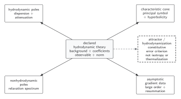
Transient sectors can control factorial large-order behavior and motivate a resummation or reduced slow manifold, but neither relation is automatic. An attractor is established only for stated variables, initial-data families, and a resolved time window. Hydrodynamization means that selected observables are described by the constitutive approximation within tolerance; it does not imply pressure isotropy or microscopic thermal equilibrium. The diagram shows independent evidence channels.

In text: identify transient decay rates, derive or measure the late-time gradient coefficients, test their asymptotics and resummation ambiguity, and compare the resummed result with many evolutions in a fixed observable and clock. Record the model, truncation, normalization, initial-data basin, and error tolerance for every collapse claim.

Exercise

For the solvable relaxation model, estimate the optimal truncation order of the series for $f(w)$ and the size of the least term at large $w$. Explain why it matches the transient scale.

Solution

The magnitude of the $n$th term is

$$t_n=\frac{n!}{w^n},$$

and successive terms obey

$$\frac{t_{n+1}}{t_n}=\frac{n+1}{w}.$$

The terms decrease until $n+1\simeq w$, so the optimal truncation is near $n_\star\simeq w-1$. Stirling’s approximation gives

$$t_{n_\star} \sim \sqrt{2\pi w}\,e^{-w}$$

up to powers that depend on the precise integer choice. The exponentially small scale $e^{-w}=e^{-\tau/\tau_R}$ is the homogeneous relaxation mode omitted by every finite power series. The extra factor $w$ in the lateral Borel ambiguity reflects the chosen normalization $f=\tau\Phi/A$.

Common pitfalls

Calling any preferred numerical solution the attractor. State the selection rule and demonstrate convergence of a nontrivial initial family.

Equating divergence with failure. A divergent asymptotic series can be highly accurate when optimally truncated; the exponentially small sectors set its limit.

Reading every Borel singularity as one microscopic particle. Singularities may arise from collective modes, nonlinear combinations, analytic continuation, or the chosen observable. An independent spectrum is needed.

Using auxiliary frame variables in a cross-theory plot. Compare invariant stress-tensor observables or provide the frame map.

Calling hydrodynamization thermalization. Constitutive predictivity can precede isotropy and microscopic equilibration.

Chapter synthesis

The chapter’s logic is now complete. Dissipative transport fixes the infrared attenuation; frame-invariant combinations identify the physical data; conventional relativistic Navier–Stokes exposes why damping is not enough; transient and BDNK formulations modify the exact principal structure in different ways; strong hyperbolicity and theorem hypotheses determine what can be claimed about the Cauchy problem; attractors organize the decay of nonhydrodynamic information without erasing model dependence.

References

• Denicol, Gabriel S., and Jorge Noronha. 2016. “Divergence of the Chapman–Enskog Expansion in Relativistic Kinetic Theory.” Physical Review D 94: 074040. DOI. Open PDF.

• Heller, Michal P., Romuald A. Janik, and Przemysław Witaszczyk. 2013. “Hydrodynamic Gradient Expansion in Gauge Theory Plasmas.” Physical Review Letters 110: 211602. DOI. Open PDF.

• Heller, Michal P., and Michał Spaliński. 2015. “Hydrodynamics Beyond the Gradient Expansion: Resurgence and Resummation.” Physical Review Letters 115: 072501. DOI. Open PDF.

• Soloviev, Alexander. 2022. “Hydrodynamic Attractors in Heavy Ion Collisions: A Review.” European Physical Journal C 82: 319. DOI. Open PDF.