Two-Time Green Functions and Self-Energies

A closed nonequilibrium evolution needs the full pair-time dependence of both the statistical correlator $F(x,y)$ and the spectral correlator $\rho(x,y)$. The component structure is developed in Danielewicz 1984, §§ 2–3. A single occupation function is not equivalent data; all approximation enters through the initial state, regulator, and self-energy closure.

Required background. Review causal and statistical propagators for the $F/\rho$ decomposition and Schwinger–Dyson identities for the functional identity behind Dyson’s equation.

Helpful background. Initial density matrices explain how preparation data enter at the initial contour boundary.

Contour equation and independent components

Let $\mathcal C$ run forward from $t_0$ to a return time and backward to $t_0$. For a real scalar field define

$$G_{\mathcal C}(x,y)=\langle T_{\mathcal C}\phi(x)\phi(y)\rangle =F(x,y)-\frac{i}{2}\operatorname{sgn}_{\mathcal C}(x^0-y^0)\rho(x,y),$$

with $F=\tfrac12\langle\{\phi,\phi\}\rangle$ and $\rho=i\langle[\phi,\phi]\rangle$. The exact inverse relation is

$$G_{\mathcal C}^{-1}=G_{0,\mathcal C}^{-1}-\Sigma_{\mathcal C}, \qquad \int_{\mathcal C}d^{d+1}z\,G_{\mathcal C}^{-1}(x,z)G_{\mathcal C}(z,y) =\delta_{\mathcal C}(x-y).$$

The four branch components $G^{++},G^{+-},G^{-+},G^{--}$ are constrained rather than independent. Hermiticity and contour ordering reduce them to $F$ and $\rho$. Away from equilibrium these depend on $x^0$ and $y^0$ separately; replacing them by functions of $x^0-y^0$ assumes stationarity and is not an innocent change of variables.

The self-energy admits the corresponding split

$$\Sigma_{\mathcal C}(x,y) =-i\Sigma^{(0)}(x)\delta_{\mathcal C}(x-y) +\Sigma_F(x,y)-\frac{i}{2}\operatorname{sgn}_{\mathcal C}(x^0-y^0)\Sigma_\rho(x,y).$$

The local term $\Sigma^{(0)}$ shifts masses or mean fields. The nonlocal $\Sigma_F$ and $\Sigma_\rho$ generate scattering, damping, and memory. Counterterms can contribute to both the local operator and, in self-consistent approximations, the kernels; “absorbing everything into a thermal mass” generally destroys the collision physics.

From Dyson’s equation to a causal initial-value problem

Multiplying the inverse equation by $G_{\mathcal C}$ and acting with the free differential operator gives

$$\big[\Box_x+m^2+\Sigma^{(0)}(x)\big]G_{\mathcal C}(x,y) =-i\delta_{\mathcal C}(x-y) -i\int_{\mathcal C}d^{d+1}z\,\Sigma_{\mathrm{nl}}(x,z)G_{\mathcal C}(z,y),$$

for the convention above. Resolving contour order converts the contour convolution into integrals whose upper limits are $x^0$ or $y^0$. That conversion—not a quasiparticle approximation—is what makes the evolution causal. The explicit component equations are derived on the Kadanoff–Baym page.

For spatially homogeneous systems one may Fourier transform only the spatial separation,

$$F_{\mathbf p}(t,t')=\int d^d\mathbf r\,e^{-i\mathbf p\cdot\mathbf r} F(t,\mathbf x;t',\mathbf x+\mathbf r),$$

while retaining both times. This turns each momentum mode into a pair-time problem without assuming energy conservation at each vertex. A relative-time Fourier transform is a later, controlled Wigner step.

The reduction diagram locates the exact two-time objects at the start of a longer hierarchy. This page reaches the causal spectral and statistical equations; it does not yet license the Wigner, gradient, shell, or Markov steps to the right.

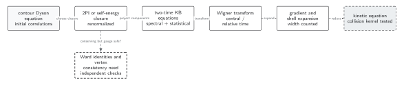
Contour Dyson equations become a closed two-time initial-value problem only after the self-energy and initial correlations are specified consistently. The spectral and statistical projections remain fully two-time objects. Every box to their right introduces a further approximation or representation change whose range must be tested rather than inferred from the Dyson equation. The diagram is schematic and not to scale.

The sections Contour equation and independent components and From Dyson’s equation to a causal initial-value problem give the text and equation equivalent of the first three boxes.

Checked free-field example

For a free homogeneous mode of frequency $\omega_{\mathbf p}=\sqrt{\mathbf p^2+m^2}$ in a Gaussian state with occupation $n_{\mathbf p}$ and no anomalous coherence,

$$F_{\mathbf p}(t,t')=\frac{n_{\mathbf p}+\tfrac12}{\omega_{\mathbf p}} \cos\!\big[\omega_{\mathbf p}(t-t')\big], \qquad \rho_{\mathbf p}(t,t')=\frac{\sin\!\big[\omega_{\mathbf p}(t-t')\big]}{\omega_{\mathbf p}}.$$

Both solve $(\partial_t^2+\omega_{\mathbf p}^2)X=0$. The spectral function obeys $\rho(t,t)=0$ and $\partial_t\rho(t,t')|_{t=t'}=1$, independent of $n_{\mathbf p}$; the statistical function carries state information through $F(t,t)=(n+1/2)/\omega$. This directly disproves the idea that one of the two functions determines the other away from KMS equilibrium.

Assumptions and failure tests

• Contour and state. State the initial time, any imaginary preparation segment, and all boundary cumulants. Omitting a correlated boundary term can masquerade as early-time damping.
• Hermiticity. Check $F(x,y)=F(y,x)$ and $\rho(x,y)=-\rho(y,x)$ at every numerical step. Violations indicate sign, quadrature, or storage errors.
• Local versus nonlocal structure. Vary the renormalization prescription and verify that counterterm changes do not alter renormalized observables within the claimed accuracy.
• No premature stationarity. Test dependence on both center and relative time before fitting a frequency-space spectral form.

Exercise

Show that the free correlators above obey the canonical equal-time conditions and reconstruct $n_{\mathbf p}$ from $F_{\mathbf p}(t,t)$ and $\partial_t\partial_{t'}F_{\mathbf p}(t,t')|_{t=t'}$.

Solution

The sine form gives $\rho(t,t)=0$ and $\partial_t\rho|_{t=t'}=\cos 0=1$. Moreover $F(t,t)=(n+1/2)/\omega$ and $\partial_t\partial_{t'}F|_{t=t'}=\omega(n+1/2)$. Hence $\omega^2=(\partial_t\partial_{t'}F)/F$ and $n=\sqrt{F\,\partial_t\partial_{t'}F}-1/2$. In an interacting state this formula is only an effective quasiparticle diagnostic, not an exact occupation number.

Continue

Use 2PI effective actions to generate a self-consistent $\Sigma[F,\rho]$, then derive its causal evolution on the Kadanoff–Baym page.

References

• Danielewicz, P. (1984). “Quantum Theory of Nonequilibrium Processes, I.” Annals of Physics 152, 239–304. DOI.
• Kadanoff, L. P., and Baym, G. (1962). Quantum Statistical Mechanics. New York: W. A. Benjamin. Internet Archive record.
• Schwinger, J. (1961). “Brownian Motion of a Quantum Oscillator.” Journal of Mathematical Physics 2, 407–432. DOI.