Thermal Propagators and Spectral Representations

In equilibrium, one spectral density determines the Wightman, retarded, advanced, time-ordered, and Euclidean two-point functions once the operator, state, grading, normalization, and contact terms are fixed. KMS supplies the thermal occupation factors; causality supplies retarded analyticity. Poles describe isolated long-lived modes only when they are actually present, while multiparticle and medium processes produce cuts and broad structure.

Compatible thermal spectral representations in real and imaginary time are reviewed in Landsman and van Weert 1987, §§ 2.3–2.5, pp. 167–191.

Required background. Thermal Density Operators and the KMS Condition supplies detailed balance. Imaginary Time and Matsubara Frequencies fixes the Euclidean modes. Helpful background. The Källén–Lehmann Representation gives the vacuum positive-metric prototype.

One spectral object

For a neutral bosonic operator $\mathcal O$, define

$$\rho(x)=\langle[\mathcal O(x),\mathcal O(0)]\rangle_\beta, \qquad \rho(p)=\int\mathrm d^d x\,e^{+ip\cdot x}\rho(x).$$

The global Fourier convention gives $p\cdot x=p^0t-\mathbf p\cdot\mathbf x$. Define

$$\begin{aligned} G^>(x)&=\langle\mathcal O(x)\mathcal O(0)\rangle,\\ G^<(x)&=\langle\mathcal O(0)\mathcal O(x)\rangle,\\ G_R(x)&=-i\theta(t)\rho(x),\\ G_A(x)&=+i\theta(-t)\rho(x). \end{aligned}$$

Then

$$\rho(\omega,\mathbf p)=G^>(\omega,\mathbf p)-G^<(\omega,\mathbf p),$$

and KMS gives

$$G^>(\omega,\mathbf p)=e^{\beta\omega}G^<(\omega,\mathbf p).$$

Therefore

$$G^<(\omega)=n_B(\omega)\rho(\omega), \qquad G^>(\omega)=[1+n_B(\omega)]\rho(\omega),$$

where $n_B(\omega)=(e^{\beta\omega}-1)^{-1}$ is understood distributionally for either sign of $\omega$. The symmetrized correlator

$$F(\omega)=\frac12(G^>+G^<) =\frac12\coth\!\left(\frac{\beta\omega}{2}\right)\rho(\omega)$$

is the equilibrium fluctuation–dissipation relation in this normalization.

Causal and Euclidean representations

For complex $z$ off the real axis and after any required subtractions, define the common Cauchy transform

$$\mathcal G(z,\mathbf p)= \int_{-\infty}^{\infty}\frac{\mathrm d\omega'}{2\pi} \frac{\rho(\omega',\mathbf p)}{z-\omega'}.$$

Its upper and lower boundary values are $G_R(\omega,\mathbf p)=\mathcal G(\omega+i0,\mathbf p)$ and $G_A(\omega,\mathbf p)=\mathcal G(\omega-i0,\mathbf p)$. Thus

$$\rho(\omega,\mathbf p)=-2\operatorname{Im}G_R(\omega+i0,\mathbf p)$$

for the displayed retarded sign. The advanced function is the opposite boundary value for a Hermitian channel.

For $0<\tau<\beta$, the Euclidean correlator is

$$G_E(\tau,\mathbf p)= \int_{-\infty}^{\infty}\frac{\mathrm d\omega}{2\pi} \frac{e^{-\omega\tau}}{1-e^{-\beta\omega}} \rho(\omega,\mathbf p).$$

For nonzero Matsubara frequencies its coefficients obey

$$G_E(i\omega_n,\mathbf p)= \int\frac{\mathrm d\omega'}{2\pi} \frac{\rho(\omega',\mathbf p)}{\omega'-i\omega_n} =-\mathcal G(i\omega_n,\mathbf p).$$

For $n>0$, this is the upper-half-plane continuation associated with $G_R$; for $n<0$, it is the lower-half-plane continuation associated with $G_A$. The bosonic zero mode requires a separately declared static limit whenever the origin is nonanalytic. The explicit Euclidean minus sign is a convention bridge, not new physics. A source defining $G_R=+i\theta(t)\langle[\mathcal O(t),\mathcal O(0)]\rangle$ changes it together with the spectral sign.

Free scalar round trip

For $E_{\mathbf p}=\sqrt{\mathbf p^2+m^2}$,

$$\rho_0(\omega,\mathbf p) =2\pi\operatorname{sgn}(\omega) \delta(\omega^2-E_{\mathbf p}^2).$$

The dispersion integral gives

$$G_R(\omega,\mathbf p)= \frac1{(\omega+i0)^2-E_{\mathbf p}^2},$$

while the Euclidean integral gives

$$G_E(i\omega_n,\mathbf p)= \frac1{\omega_n^2+E_{\mathbf p}^2}.$$

Transforming to imaginary time recovers the Bose-weighted result on the Matsubara page. This round trip checks the delta-function normalization, retarded sign, Euclidean minus sign, and occupation factors independently.

Interactions replace the delta functions by shifted poles, finite-width resonances, and cuts. A Breit–Wigner fit may be useful in a controlled quasiparticle regime, but a broad bump is not by itself proof of a pole on a specified analytic sheet.

Fermions, charge, and contact terms

For fermionic fields use the anticommutator spectral function appropriate to the spinor two-point function; KMS contains Fermi factors and matrix numerator structure. For non-Hermitian charged operators, $\rho_{AB}$ and $\rho_{BA}$ are distinct and the chemical potential changes detailed balance. Gauge-fixed elementary fields may live in an indefinite state space, so positive scalar spectral intuition does not automatically apply.

Polynomial contact terms can be invisible in $\rho$ away from infinity yet contribute to Euclidean correlators or sum rules. Dispersion relations must include the number of subtractions required by ultraviolet growth.

The shared equilibrium convention table records these distinctions. Exact continuation is developed on Exact Euclidean–Real-Time Analytic Continuation.

The schematic below organizes the relationships used on this page. Inspect it with this question in mind: What connects thermal correlators, spectral densities, exact continuation, and finite-data reconstruction?

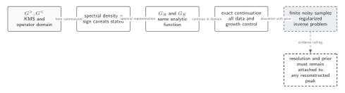
KMS and the commutator determine compatible Euclidean and retarded representations; exact analytic continuation is unique under its hypotheses, whereas reconstructing a spectrum from finite noisy data is an ill-posed inference problem. Solid connections show the primary relation; dashed outlines or arrows mark qualifications and failure boundaries. The diagram is schematic and not to scale.

The surrounding discussion supplies the relevant equations and checks in text form; the figure is a navigational summary.

Exercise

Use the free spectral function above to verify $G^>(\omega)=e^{\beta\omega}G^<(\omega)$ at both $\omega=\pm E_{\mathbf p}$.

Solution

At $+E$, $G^<$ has weight $n_B(E)$ and $G^>$ has $1+n_B(E)=e^{\beta E}n_B(E)$. At $-E$, $\rho$ changes sign and $n_B(-E)=-[1+n_B(E)]$, so $G^<(-E)$ and $G^>(-E)$ interchange with the required factor $e^{-\beta E}$. The negative-frequency part is essential for the relation.

References

• Landsman, N. P., and Ch. G. van Weert. “Real- and Imaginary-Time Field Theory at Finite Temperature and Density.” Physics Reports 145, nos. 3–4 (1987): 141–249. doi:10.1016/0370-1573(87)90121-9.
• Le Bellac, Michel. Thermal Field Theory. Cambridge: Cambridge University Press, 1996. doi:10.1017/CBO9780511721700.
• Martin, Paul C., and Julian Schwinger. “Theory of Many-Particle Systems. I.” Physical Review 115, no. 6 (1959): 1342–1373. doi:10.1103/PhysRev.115.1342.