Langevin Field Equations and Noise

A Langevin field equation combines deterministic relaxation of chosen slow variables with random forcing from unresolved degrees of freedom. For equilibrium Model A, the noise strength is fixed by the mobility and temperature; choosing it independently changes the stationary measure.

Required background. Use stochastic processes and correlation functions and Gaussian fluctuations and free energy.

Helpful background. KMS and fluctuation–dissipation gives the quantum equilibrium relation from which a classical white-noise limit may descend.

Model-A relaxation and noise

For a nonconserved scalar order parameter, Model-A dynamics in the classification of Hohenberg and Halperin 1977, § III.A is

$$\partial_t\phi(t,\mathbf x) =-\Gamma\frac{\delta\mathcal F[\phi]}{\delta\phi(\mathbf x)} +\xi(t,\mathbf x),$$

with $\Gamma>0$. Additive Gaussian white noise has

$$\langle\xi(t,\mathbf x)\rangle=0, \qquad \langle\xi(t,\mathbf x)\xi(t',\mathbf x')\rangle =2\Gamma T\,\delta(t-t')\delta^{(d)}(\mathbf x-\mathbf x').$$

The factor of two and every delta function belong to the definition. In the continuum, white noise has arbitrarily short wavelengths, so interacting stochastic field theory requires a spatial regulator and renormalized parameters. A lattice noise variance contains inverse cell volume and timestep; omitting either changes the continuum limit.

The sign of the drift is checked by the deterministic free-energy change:

$$\frac{d\mathcal F}{dt} =-\Gamma\int d^dx \left(\frac{\delta\mathcal F}{\delta\phi}\right)^2\le0$$

when noise is absent.

The schematic starts one step before the equation: the slow variables, noise statistics, and stochastic calculus must be declared before a Langevin model has a definite probability or response interpretation.

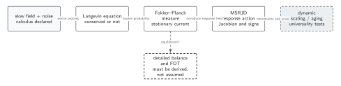
A Langevin equation defines a stochastic process only together with its field content, noise correlators, stochastic prescription, and boundary conditions. The associated Fokker–Planck and response descriptions must agree with those choices. Noise amplitude does not by itself establish thermal equilibrium: detailed balance and fluctuation–dissipation occupy the conditional dashed branch. The diagram is schematic and not to scale.

The sections Model-A relaxation and noise, Checked Gaussian solution, and Stochastic and kinetic closure validity provide the text and equation equivalent, with validation conditions, for the first three boxes.

Checked Gaussian solution

Take

$$\mathcal F=\frac12\int\frac{d^dk}{(2\pi)^d} (r+k^2)|\phi_{\mathbf k}|^2.$$

Each Fourier mode obeys an Ornstein–Uhlenbeck equation

$$\dot\phi_{\mathbf k} =-\omega_k\phi_{\mathbf k}+\xi_{\mathbf k}, \qquad \omega_k=\Gamma(r+k^2).$$

Its solution is

$$\phi_{\mathbf k}(t) =e^{-\omega_k(t-t_0)}\phi_{\mathbf k}(t_0) +\int_{t_0}^{t}ds\,e^{-\omega_k(t-s)}\xi_{\mathbf k}(s).$$

The retarded response to a field $h$ coupled through $\mathcal F-h\phi$ is

$$R_k(t-t')=\Gamma\theta(t-t')e^{-\omega_k(t-t')}.$$

At late times,

$$\langle|\phi_{\mathbf k}|^2\rangle_{\mathrm{st}} =\frac{T}{r+k^2},$$

which is precisely the Gaussian Gibbs covariance. If the noise amplitude were $2D$ instead, the effective covariance would be $D/[\Gamma(r+k^2)]$; equilibrium at temperature $T$ requires $D=\Gamma T$.

This result is an ensemble average. A single realization remains noisy and does not equal the covariance; time averaging equals ensemble averaging only with ergodicity and a sufficiently long observation.

Stochastic and kinetic closure validity

Minimum record and failure test for stochastic and kinetic reductions

Element	Required record	Independent check	Failure signal	Licensed inference
Stochastic prescription	Itô, Stratonovich, or other discretization; equal-time response rule	Translate the drift between two prescriptions	Stationary measure changes under an unrecorded convention	Dynamics in the declared stochastic calculus
Regulator	Spatial lattice/cutoff, timestep, boundary conditions, renormalized parameters	Cutoff and step refinement at fixed physical inputs	Covariance or drift scales with cell size	Regulator-independent observables in the tested window
Noise covariance	Mean, full two-point kernel, Gaussian or higher cumulants, conserved structure	Measure generated noise in Fourier and real space	Wrong delta normalization, negative spectrum, or lost zero mode	The specified effective noise process
Stationary measure	Probability current, normalization, support, boundary flux	Fokker–Planck substitution and long-run histogram	Formal zero mode is nonnormalizable or carries irreversible current	Stationarity; equilibrium only if detailed balance also holds
Response convention	Source coupling, response-field contour, Jacobian, contact prescription	Finite-difference response versus MSRJD correlator	Advanced support or a missing equal-time contact	Causal response under the declared convention
Collision invariants	Complete reaction set and conserved charge/momentum vectors	Analytic and discrete collision moments	Charge or energy drift that survives refinement	Conservation by the stated kinetic kernel
Closure order	Gradient, quasiparticle, memory, moment, matrix, and coupling counting	Add the first omitted term or enlarge the basis	Target changes at the same order as the result	Accuracy no stronger than the demonstrated hierarchy
Positivity	Scalar bounds or matrix eigenvalue condition; limiter intervention	Monitor bounds and weighted clipped moments	Limiter controls the observable or fermionic bound is exceeded	Positive effective state only in the tested discretization/regime
Convergence	Independent step, grid, cutoff, volume, tail, memory, and solver studies	Observed order and benchmark comparison	Only a combined refinement or fitted parameter stabilizes the curve	Numerical solution of the declared effective equations
Failure boundary	Scale ratios, omitted slow variables, driving, evidence range	Cross the boundary deliberately in a controlled test	No qualitative change where the approximation predicts breakdown	Model-dependent prediction inside the validated domain

This table is reused by Fokker–Planck evolution, the MSRJD functional, generalized noise, collision kernels, moment closures, and kinetic validity.

Failure tests

• Measure the generated noise covariance with all lattice factors.
• Verify deterministic free-energy descent and stationary Gibbs covariance.
• Vary initial conditions and distinguish transient from stationary averages.
• Raise the ultraviolet cutoff while renormalizing the effective functional.
• Test white/Markov assumptions against the eliminated correlation time.
• State whether the slow variable is conserved; conserved dynamics has a different drift and noise kernel.

Exercise

Compute the finite-time variance of one Gaussian mode initialized at deterministic value $\phi_0$.

Solution

The mean is $e^{-\omega t}\phi_0$. With noise strength $2\Gamma T$, the variance is $2\Gamma T\int_0^t ds\,e^{-2\omega(t-s)} =T[1-e^{-2\omega t}]/(r+k^2)$, which approaches the Gibbs covariance.

Continue

Derive probability flow on Fokker–Planck evolution and causal response on the MSRJD functional.

References

• Hohenberg, P. C., and Halperin, B. I. (1977). “Theory of Dynamic Critical Phenomena.” Reviews of Modern Physics 49, 435–479. DOI.
• Langevin, P. (1908). “Sur la théorie du mouvement brownien.” Comptes Rendus de l’Académie des Sciences 146, 530–533. Gallica scan.