Ideal Relativistic Hydrodynamics

Ideal relativistic hydrodynamics is the zeroth-derivative closure of energy–momentum and charge conservation. Local isotropy fixes the perfect-fluid tensors; the equation of state closes the nonlinear Euler equations. The theory is nondissipative for smooth solutions, but it can form shocks, and relativistic causality imposes an equation-of-state condition beyond ordinary thermodynamic stability.

Required background. Conservation Laws and Hydrodynamic Fields fixes the Ward identities and decomposition. Hydrodynamic Frames and Constitutive Data explains why frame ambiguity begins only in derivative corrections to the ideal tensors.

Helpful background. Symbols, Characteristics, and PDE Type supplies the characteristic language used for sound and shocks.

Perfect-fluid constitutive data

For one conserved $U(1)$ charge and no external sources,

$$T_{(0)}^{\mu\nu} = \epsilon u^\mu u^\nu+pP^{\mu\nu}, \qquad J_{(0)}^\mu=n\,u^\mu,$$

where $P^{\mu\nu}=u^\mu u^\nu-g^{\mu\nu}$ and $u^2=1$. Equivalently,

$$T_{(0)}^{\mu\nu} = (\epsilon+p)u^\mu u^\nu-pg^{\mu\nu}.$$

The equation of state may be given as $p=p(\epsilon,n)$ or parametrically by $p(T,\mu)$, $\epsilon(T,\mu)$, and $n(T,\mu)$. It is microscopic input. Conservation and Lorentz symmetry do not determine it.

The thermodynamic relations are

$$\mathrm d\epsilon=T\,\mathrm ds+\mu\,\mathrm dn, \qquad \mathrm dp=s\,\mathrm dT+n\,\mathrm d\mu, \qquad w:=\epsilon+p=Ts+\mu n.$$

Relativistic Euler equations

Project $\nabla_\mu T^{\mu\nu}=0$ along $u_\nu$ and into the rest space. With $D=u^\mu\nabla_\mu$, $\theta=\nabla_\mu u^\mu$, and $a^\mu=Du^\mu$,

$$D\epsilon+w\theta=0,$$ $$wa^\mu+\nabla_\perp^\mu p=0.$$

Charge conservation gives

$$Dn+n\theta=0.$$

These are respectively energy balance, relativistic Euler acceleration, and charge advection. The signs can be checked in the local rest frame:

$$\partial_t\delta\epsilon+w\,\boldsymbol\nabla\!\cdot\!\mathbf v=0, \qquad w\,\partial_t\mathbf v+\boldsymbol\nabla\delta p=0.$$

Combining the energy and charge equations with the first law yields

$$Ds+s\theta=0.$$

For $n\ne0$,

$$D\!\left(\frac{s}{n}\right)=0,$$

so the entropy per particle is advected along each smooth fluid worldline. This is not a microscopic entropy conservation law and fails across entropy-producing shocks or once dissipative terms are included.

Characteristic sound speed

Linearize about a homogeneous equilibrium. For a propagating longitudinal perturbation, charge and energy conservation imply

$$\delta n=\frac{n}{w}\delta\epsilon.$$

Writing

$$\delta p = p_\epsilon\,\delta\epsilon+p_n\,\delta n,$$

the longitudinal equations give

$$\omega^2=c_s^2k^2, \qquad c_s^2 = p_\epsilon+\frac{n}{w}p_n = \left(\frac{\partial p}{\partial\epsilon}\right)_{s/n}.$$

The thermodynamic projection and its charged-fluid characteristic interpretation are derived in Romatschke and Romatschke 2019, §§2.1–2.3.

Thermodynamic stability requires a positive susceptibility matrix and gives $c_s^2\ge0$ in the ordinary stable region. Relativistic characteristic causality additionally requires

$$c_s^2\le1.$$

The upper bound does not follow from convexity alone; it is a restriction on a relativistic equation of state. At $c_s^2=0$ strict hyperbolicity can degenerate, and at a phase boundary the correct weak-solution problem may require more variables.

Homogeneous longitudinal expansion

For boost-invariant longitudinal flow, proper time is $\tau=\sqrt{t^2-z^2}$ and the ideal conservation law reduces to

$$\frac{\mathrm d\epsilon}{\mathrm d\tau} = -\frac{\epsilon+p}{\tau}.$$

If $p=c_s^2\epsilon$ with constant $c_s^2$,

$$\epsilon(\tau) = \epsilon(\tau_0) \left(\frac{\tau_0}{\tau}\right)^{1+c_s^2}.$$

For a conformal fluid in four dimensions, $c_s^2=1/3$ and $\epsilon\propto\tau^{-4/3}$. Substitution back into the conservation equation verifies both the exponent and sign. The solution is an ideal benchmark, not evidence that a collision has thermalized or that viscous corrections are negligible.

Nonrelativistic limit

Take $u^\mu=(1+\tfrac12\mathbf v^2,\mathbf v)+O(v^3)$ and split

$$\epsilon=\rho_m+\varepsilon_{\mathrm{int}}, \qquad p,\varepsilon_{\mathrm{int}}\ll\rho_m.$$

The spatial Euler equation becomes

$$\rho_m \left( \partial_t+\mathbf v\!\cdot\!\boldsymbol\nabla \right)\mathbf v +\boldsymbol\nabla p=0,$$

while charge or mass conservation reduces to the ordinary continuity equation. The rest-mass contribution cancels appropriately between energy and momentum; dropping it before taking the limit gives the wrong inertia.

Shocks and weak solutions

Even smooth initial data can steepen. Across a discontinuity with normal covector $n_\mu$, distributional conservation requires the Rankine–Hugoniot conditions

$$n_\mu[T^{\mu\nu}]=0, \qquad n_\mu[J^\mu]=0,$$

where $[\,\cdot\,]$ is the jump. These conditions do not select the physical branch by themselves. An entropy condition or viscous limiting procedure is required. Thus “ideal” means no constitutive dissipation in smooth regions, not that every weak solution is reversible.

Rezzolla and Zanotti derive the relativistic Euler characteristics and shock conditions in a consistent initial-value formulation Rezzolla and Zanotti 2013, chs. 2 and 4.

The right-hand end of the schematic places the ideal equations in the larger constitutive construction. Inspect the transition from constitutive tensors to modes while retaining the distinction between the nonlinear Euler system derived here and its later linearization.

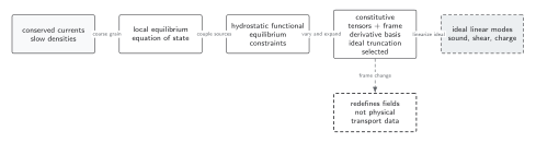
At zeroth derivative order, the equation of state closes the conserved stress and current and yields the nonlinear relativistic Euler equations. Linearizing that ideal truncation produces sound plus degenerate transverse and charge sectors; shocks and weak solutions require additional analysis. The diagram is schematic and does not depict nonlinear characteristics, shock formation, or dissipation.

In text: set dissipative corrections to zero, project $\nabla_\mu T^{\mu\nu}=F^{\nu\lambda}J_\lambda$ along and transverse to $u^\mu$, supplement it with charge conservation and an equation of state, and only then linearize about a chosen equilibrium.

Exercise

For $p=\epsilon/3$ and zero charge, verify the sound characteristics and the Bjorken energy law.

Solution

The equation of state gives $c_s^2=\mathrm dp/\mathrm d\epsilon=1/3$, hence $\omega=\pm k/\sqrt3$. The homogeneous expansion equation is

$$\frac{\mathrm d\epsilon}{\mathrm d\tau} =-\frac{4\epsilon}{3\tau}.$$

Integrating gives $\epsilon=C\tau^{-4/3}$. Direct differentiation yields $-4C\tau^{-7/3}/3$, equal to $-4\epsilon/(3\tau)$.

Common pitfalls

Inferring the equation of state from hydrodynamics. Hydrodynamics propagates thermodynamic input; it does not calculate $p(\epsilon,n)$.

Equating entropy advection with absence of shocks. Smooth ideal evolution conserves entropy per particle, while admissible shocks produce entropy.

Calling $c_s^2>0$ a complete causality test. A relativistic perfect fluid also needs $c_s^2\le1$ and a well-defined initial-value domain. Dissipative theories need additional characteristic tests.

Where this leads

Sound, Shear, and Charge Modes diagonalizes all ideal sectors and identifies the zero modes that become diffusive after dissipation. Relativistic Dissipative Hydrodynamics adds the first attenuation terms.

References

• Rezzolla, Luciano, and Olindo Zanotti. 2013. Relativistic Hydrodynamics. Oxford University Press. DOI.

• Romatschke, Paul, and Ulrike Romatschke. 2019. Relativistic Fluid Dynamics In and Out of Equilibrium. Cambridge University Press. DOI.