Free Energy and Pressure in Loop Expansion

The logarithm of the thermal partition function is the sum of connected vacuum diagrams. Dividing by $\beta V$ gives the free-energy density, and pressure is its negative after a declared vacuum normalization. Symmetry factors, counterterm insertions, and zero-mode reorganization are part of the loop order; thermodynamic derivatives provide an independent consistency check.

The thermodynamic loop organization and vacuum-diagram normalization used here are presented in Kapusta and Gale 2006, chs. 2–3.

Required background. Thermal Sum-Integrals and Vacuum Subtraction fixes the trace logs. Thermal Counterterms and Renormalization-Group Invariance fixes subtraction. Connected, Disconnected, and Vacuum Diagrams supplies the linked-cluster theorem.

Linked-cluster expansion

Write $S_E=S_0+S_{\mathrm{int}}$. Then

$$Z=Z_0\left\langle e^{-S_{\mathrm{int}}}\right\rangle_0,$$

and

$$\log Z=\log Z_0 -\langle S_{\mathrm{int}}\rangle_0 +\frac12\langle S_{\mathrm{int}}^2\rangle_{0,c} -\cdots.$$

Disconnected vacuum pieces exponentiate and cancel from $\log Z$ except through their connected components. The free-energy density and pressure are

$$f=-\frac{T}{V}\log Z, \qquad p=\frac{T}{V}\log Z=-f.$$

Every closed diagram supplies $\beta V$ from translation invariance; forgetting to divide by it gives an extensive quantity where a density was intended.

Massless scalar pressure at first interaction order

For one real scalar with

$$S_{\mathrm{int}}= \int_0^\beta\mathrm d\tau\int_V\mathrm d^3x\, \frac{\lambda}{4!}\phi^4,$$

Wick’s theorem gives $\langle\phi^4\rangle_0=3G_0(0)^2$. After vacuum subtraction,

$$G_0(0)_{\mathrm{th}}=\frac{T^2}{12}.$$

Therefore

$$\Delta f =\frac{\lambda}{4!}\,3 \left(\frac{T^2}{12}\right)^2 =\frac{\lambda T^4}{1152},$$

and

$$p(T)=\frac{\pi^2T^4}{90} -\frac{\lambda T^4}{1152} +O(\lambda^{3/2}).$$

The factor $3/4!=1/8$ is the figure-eight symmetry factor. The next correction is written $O(\lambda^{3/2})$, not $O(\lambda^2)$, because scalar zero-mode rings generate a nonanalytic contribution after screening.

This formula uses the renormalized coupling in a declared scheme and a vacuum pressure set to zero. A massive theory retains vacuum and thermal cross terms whose divergences are canceled by counterterm diagrams; keeping only the thermal piece inside each diagram can spoil those cancellations.

Thermodynamic consistency

For a pressure $p(T)$ at zero chemical potential,

$$s=\frac{\partial p}{\partial T}, \qquad \epsilon=-p+Ts, \qquad \epsilon-3p=T^5\frac{\mathrm d}{\mathrm dT} \left(\frac{p}{T^4}\right)$$

in four spacetime dimensions. If $\lambda$ runs, its implicit $T$ dependence through the chosen scale contributes to the trace anomaly. Differentiating while treating a running or thermally matched parameter as constant gives an inconsistent energy density.

The same thermodynamic quantities can be obtained from stress-tensor expectation values. Agreement checks diagram normalization, counterterms, and derivatives. Composite stress-tensor improvement and vacuum terms must be matched between the two routes.

Error and infrared boundaries

Scale variation, the size of the last known term, and comparison among consistent reorganizations can diagnose truncation. None is a rigorous uncertainty bound near an infrared breakdown. Before quoting a loop-order pressure:

• verify all connected topologies and symmetry factors;
• include vacuum-energy and coupling counterterms at the same order;
• separate hard and zero-mode contributions without overlap;
• test RG invariance through the claimed order;
• check $s$ and $\epsilon$ by differentiation and operator expectation; and
• state the first nonanalytic or nonperturbative contribution not computed.

The schematic below organizes the relationships used on this page. Inspect it with this question in mind: How does a thermal loop calculation pass from scale counting to a physical observable?

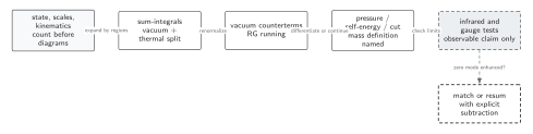
Thermal power counting chooses hard and soft regions; sum-integrals are split into vacuum and thermal parts, vacuum counterterms renormalize them, and mass, width, infrared, RG, and gauge checks bound the final observable. Solid connections show the primary relation; dashed outlines or arrows mark qualifications and failure boundaries. The diagram is schematic and not to scale.

The surrounding discussion supplies the relevant equations and checks in text form; the figure is a navigational summary.

Exercise

Why does replacing $G_0(0)$ by only its thermal part inside the massless first-order scalar diagram give the correct displayed finite term but fail as a general renormalization prescription?

Solution

In dimensional regularization the massless vacuum tadpole is scaleless and vanishes, so the shortcut happens to reproduce $\lambda T^4/1152$. With mass, external scales, or higher-loop subdivergences, vacuum pieces are nonzero and combine with counterterms and thermal factors. Dropping them diagram by diagram can remove required subdivergences or finite normalization terms.

References

• Arnold, Peter, and Cheng-xing Zhai. “The Three-Loop Free Energy for High Temperature QED and QCD with Fermions.” Physical Review D 51, no. 4 (1995): 1906–1918. doi:10.1103/PhysRevD.51.1906.
• Kapusta, Joseph I., and Charles Gale. Finite-Temperature Field Theory: Principles and Applications. 2nd ed. Cambridge: Cambridge University Press, 2006. doi:10.1017/CBO9780511535130.