Correlations, Susceptibilities, and Correlation Lengths

Static response and spatial correlation are two views of the same equilibrium fluctuations. A susceptibility is a source derivative and, after contact terms and normalizations are matched, the integral of a connected correlation function. A correlation length can be read from asymptotic decay, a screening pole, or a second moment, but these estimators agree only when one isolated long-distance scale dominates. None is automatically a real-time quasiparticle mass.

The scaling relations among correlations, susceptibilities, and correlation lengths are reviewed with their critical assumptions in Fisher 1967, pp. 615–730.

Required background. Partition Functions and Thermodynamic Response supplies the source derivatives. Connected Correlators and Cumulants fixes connected normalization. Helpful background. Critical Exponents, Scaling Relations, and Hyperscaling Caveats develops the scaling limit used near criticality.

Connected correlations and response

For a translation-invariant scalar observable $\mathcal O(\mathbf x)$, define

$$C(\mathbf x)= \langle\mathcal O(\mathbf x)\mathcal O(\mathbf0)\rangle -\langle\mathcal O\rangle^2.$$

Couple a uniform source through $H_h=H-h\int_V\mathrm d^{d-1}x\,\mathcal O$. Then

$$\chi =\frac{\partial\langle\mathcal O\rangle}{\partial h} =\beta\int_V\mathrm d^{d-1}x\,C(\mathbf x),$$

where $\langle\mathcal O\rangle$ denotes the spatially averaged density. If the source also changes the operator or action explicitly, a contact term must be added. On a finite periodic lattice the same identity holds as a sum, with the zero mode and volume normalization stated explicitly.

The structure factor is

$$S(\mathbf k)=\int\mathrm d^{d-1}x\, e^{-i\mathbf k\cdot\mathbf x}C(\mathbf x).$$

Although the global Fourier convention uses $e^{+ip\cdot x}$, this spatial definition is written explicitly and is even in $\mathbf k$ for a parity-invariant real channel. With the convention above, $\chi=\beta S(\mathbf0)$ after any required contact subtraction.

Exponential, screening, and second-moment lengths

If one isolated screening state controls large separation,

$$C(r)\sim A\,r^{-(d-2)/2}e^{-r/\xi_{\mathrm{exp}}}.$$

Equivalently $S(\mathbf k)$ has a nearest singularity at $\mathbf k^2=-\xi_{\mathrm{exp}}^{-2}$. At small real momentum an Ornstein–Zernike form reads

$$S(\mathbf k)\simeq \frac{S(0)}{1+\xi_2^2\mathbf k^2+O(k^4)},$$

with second-moment length

$$\xi_2^2 =\frac{1}{2(d-1)} \frac{\int\mathrm d^{d-1}x\,\mathbf x^2 C(\mathbf x)} {\int\mathrm d^{d-1}x\,C(\mathbf x)}.$$

On a periodic lattice of extent $L$ a common estimator avoids coordinate wrapping:

$$\xi_{2,L} =\frac{1}{2\sin(\pi/L)} \left[ \frac{S(\mathbf0)}{S(\mathbf k_{\min})}-1 \right]^{1/2}, \qquad \mathbf k_{\min}=\frac{2\pi}{L}(1,0,\ldots).$$

This formula assumes an approximately isotropic single-pole small-momentum form. Direction-dependent estimators are required on anisotropic lattices; a multi-exponential channel need not yield $\xi_2=\xi_{\mathrm{exp}}$.

Gaussian check and critical scaling

For the static Gaussian functional

$$\mathcal F[\phi] =\frac12\int\mathrm d^{d-1}x \left[(\nabla\phi)^2+m_s^2\phi^2\right],$$

the covariance is

$$S(\mathbf k)=\frac{T}{\mathbf k^2+m_s^2}.$$

Therefore

$$\xi=\frac1{m_s}, \qquad \chi=\beta S(0)=\frac1{m_s^2}$$

for the displayed source normalization. This is a screening mass: it controls static spatial decay. A pole mass comes from a real-time frequency singularity, and a curvature mass from a local effective-potential Hessian. Interactions can separate all three.

Near a continuous transition, a scaling form is

$$C(r;t)\sim \frac{1}{r^{d-3+\eta}}\, \mathcal C(r/\xi), \qquad \xi\sim\lvert t\rvert^{-\nu}, \qquad \chi\sim\xi^{2-\eta}.$$

Finite volume cuts off the divergence when $\xi$ approaches $L$. Extracting a critical exponent therefore requires a joint finite-size and scaling-window analysis; fitting a large but finite $\xi$ at one volume does not establish a critical point.

Validation checklist

• Confirm that connected rather than full correlations are integrated.
• State the source sign and any contact or zero-mode subtraction.
• Compare exponential and second-moment estimators over increasing volumes.
• Vary the fit window and include more than one screening state when required.
• Test anisotropy by rotating $\mathbf k_{\min}$.
• Keep screening, curvature, pole, and damping scales distinct.
• Near criticality, demonstrate $L/\xi$ control rather than extrapolating a single volume.

The finite-volume and limit distinctions are summarized in the shared equilibrium table. Gaussian determinants and the failure of quadratic control continue on Gaussian Fluctuations and Effective Free Energy.

The schematic below organizes the relationships used on this page. Inspect it with this question in mind: How do Euclidean configurations, correlations, Gaussian fluctuations, phases, and thermodynamic limits relate?

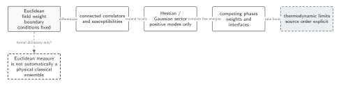
A Euclidean weight defines correlations; a positive Hessian licenses Gaussian fluctuations locally, while phase coexistence and spontaneous breaking require a separately ordered thermodynamic and source limit. Solid connections show the primary relation; dashed outlines or arrows mark qualifications and failure boundaries. The diagram is schematic and not to scale.

The surrounding discussion supplies the relevant equations and checks in text form; the figure is a navigational summary.

Exercise

For $S(k)=A/(k^2+m_1^2)+B/(k^2+m_2^2)$ with $0<m_1<m_2$ and $A,B>0$, compare the exponential and second-moment lengths.

Solution

The large-distance decay is controlled by the nearest pole, so $\xi_{\mathrm{exp}}=1/m_1$. Expanding at small $k$ gives $\xi_2^2=(A/m_1^4+B/m_2^4)/(A/m_1^2+B/m_2^2)$. Unless the light pole dominates the zero-momentum weight, $\xi_2<1/m_1$. The difference is a diagnostic of multiple scales, not a contradiction.

References

• Fisher, Michael E. “The Theory of Equilibrium Critical Phenomena.” Reports on Progress in Physics 30, no. 2 (1967): 615–730. doi:10.1088/0034-4885/30/2/306.
• Kardar, Mehran. Statistical Physics of Fields. Cambridge: Cambridge University Press, 2007. doi:10.1017/CBO9780511815881.
• Zinn-Justin, Jean. Quantum Field Theory and Critical Phenomena. 5th ed. Oxford: Oxford University Press, 2021. doi:10.1093/oso/9780198834625.001.0001.