Thermodynamic Limits, Phases, and Ensemble Equivalence

A strict thermodynamic phase is an infinite-volume concept. At finite volume with a regular action, the partition function is normally analytic and a symmetric Gibbs measure averages over symmetry-related configurations. A selected broken phase arises by taking the thermodynamic limit before removing its selecting field or boundary condition. Canonical and microcanonical ensembles become equivalent only under suitable additivity and concavity hypotheses; long-range forces and nonconcave entropy can preserve inequivalence.

The analytic finite-volume zeros underlying the phase-limit discussion were established by Lee and Yang 1952, pp. 410–419.

Required background. Partition Functions and Thermodynamic Response supplies the finite-volume potentials and convexity relations. Helpful background. Symmetry Realization and Order Parameters distinguishes invariant states from order-parameter realizations.

Finite volume is analytic, not phase-free in every practical sense

For finitely many regulated degrees of freedom and a stable integration measure,

$$Z_V(h)=\int\mathrm d\nu_V(X) \,e^{-\beta[H_V(X)-hM_V(X)]}$$

is analytic in real $h$ and $\beta$ away from singularities caused by an ill-defined measure. It can show sharp crossovers, metastable peaks, and exponentially slow tunneling, but no exact nonanalytic thermodynamic transition. Zeros of $Z_V$ lie off the real control axis and may approach it only as $V\to\infty$, which is the Lee–Yang mechanism for nonanalyticity Lee and Yang 1952.

Finite-volume data remain indispensable: scaling of susceptibilities, Binder-type cumulants, histogram barriers, and partition-function zeros can diagnose an approaching limit. The claim must nevertheless be phrased as finite-size evidence until the volume extrapolation and order of limits are controlled.

Selecting a pure phase

Suppose a $\mathbb Z_2$-symmetric system has order parameter density $m_V=\langle M_V\rangle/V$. At every finite $V$ and $h=0$, symmetry gives $m_V=0$. A positive phase is defined by

$$m_+ =\lim_{h\to0^+}\lim_{V\to\infty} \frac{\langle M_V\rangle_{V,h}}{V}.$$

Reversing the limits gives zero:

$$\lim_{V\to\infty}\lim_{h\to0} \frac{\langle M_V\rangle_{V,h}}{V}=0.$$

Boundary conditions can play the role of the selecting field. A pure phase satisfies an appropriate clustering property; a symmetric mixture of $+$ and $-$ phases generally retains long-range correlations from phase mixing even though its one-point function vanishes.

The order parameter is not itself the definition of every phase. Topological order, gauge theories, and phases distinguished by generalized symmetry or nonlocal response need their own invariant characterization. This chapter owns the limit logic, while the relevant order parameter or observable remains with its symmetry or system-specific owner.

Ensemble equivalence from convex duality

Let the density of states obey

$$\Omega_V(Ve)\asymp e^{V s(e)}.$$

The canonical free-energy density is given by the Legendre–Fenchel transform

$$\beta f(\beta)=\inf_e[\beta e-s(e)].$$

If $s(e)$ is concave and sufficiently regular, an exposed energy density is selected by $\beta=s'(e)$, and local thermodynamic observables agree between microcanonical and canonical ensembles in the limit. A linear segment of $s$ corresponds to coexistence and latent heat. If $s$ is nonconcave, the canonical transform retains only its concave envelope: some microcanonical energies are skipped, negative microcanonical heat capacity may occur, and the ensembles are inequivalent.

Short-range stable interactions are the standard setting in which additivity drives concavity. Gravitational systems, unscreened long-range interactions, nonadditive constraints, and some mean-field models fall outside that inference. Equivalence of thermodynamic potentials also need not imply identical fluctuations or large deviations at coexistence.

Limit and phase checks

Question	Required declaration	Diagnostic
Is there a phase transition?	Regulator, $V\to\infty$ sequence, control parameter	finite-size scaling or zeros approaching the real axis
Is a phase selected?	source or boundary condition and its removal order	nonzero order parameter plus clustering or another invariant criterion
Are ensembles equivalent?	additive variables and entropy concavity	matching exposed thermodynamic states and local observables
Is coexistence present?	constrained versus canonical potential	bimodality with interface scaling, not bimodality alone
Is a theorem being used?	interaction range, stability, boundary, topology	verify every hypothesis; do not infer it from a numerical plot

The broader finite-volume distinctions are collected in the shared convention and limit table.

Common pitfalls

A finite histogram called a phase. Two peaks may result from poor mixing or a finite-size crossover. Demonstrate volume scaling, relative weights, and interface suppression.

A nonconvex approximate potential called exact. The exact Legendre effective potential is convex in the thermodynamic treatment. Nonconvex coarse-grained potentials can encode metastability, but their scale and approximation must be named.

Ensemble equivalence assumed from matching means. Fluctuation and rare-event sectors can differ even where an equation of state agrees. State the observable class under comparison.

The schematic below organizes the relationships used on this page. Inspect it with this question in mind: How do Euclidean configurations, correlations, Gaussian fluctuations, phases, and thermodynamic limits relate?

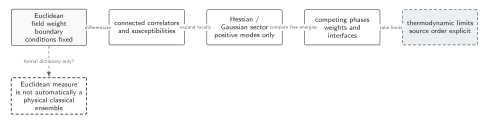
A Euclidean weight defines correlations; a positive Hessian licenses Gaussian fluctuations locally, while phase coexistence and spontaneous breaking require a separately ordered thermodynamic and source limit. Solid connections show the primary relation; dashed outlines or arrows mark qualifications and failure boundaries. The diagram is schematic and not to scale.

The surrounding discussion supplies the relevant equations and checks in text form; the figure is a navigational summary.

Exercise

Why does a finite $\mathbb Z_2$-symmetric system have $\langle M\rangle=0$ at $h=0$ even when its histogram has peaks near $\pm M_0$?

Solution

The transformation $X\mapsto-X$ preserves the measure and sends $M\mapsto-M$. Pairing configurations therefore cancels the first moment exactly. The two peaks describe large fluctuations or long-lived phase-like sectors, but a nonzero selected expectation requires $V\to\infty$ before $h\to0^\pm$ or a symmetry-breaking boundary condition.

References

• Ellis, Richard S. Entropy, Large Deviations, and Statistical Mechanics. New York: Springer, 1985. doi:10.1007/978-1-4613-8533-2.
• Lee, T. D., and C. N. Yang. “Statistical Theory of Equations of State and Phase Transitions. II. Lattice Gas and Ising Model.” Physical Review 87, no. 3 (1952): 410–419. doi:10.1103/PhysRev.87.410.
• Ruelle, David. Statistical Mechanics: Rigorous Results. Singapore: World Scientific, 1999. doi:10.1142/4090.