Quasiparticle Shell Reduction and Gradient Power Counting

A quasiparticle expansion is controlled by a joint hierarchy, not by weak coupling alone. The spectral width must be small compared with the excitation energy and every nearby branch separation; gradients must be small on the spectral correlation scale; and all terms enhanced by narrow widths, thresholds, or infrared modes must be resummed before ordinary order counting is trusted.

Required background. Use Kadanoff–Baym reduction and thermal self-energies and mass definitions.

Helpful background. Kinetic validity and breakdown turns this power counting into numerical acceptance tests.

Spectral shell and width

For a scalar retarded propagator,

$$G_R(X,p)=\frac{1}{p^2-m^2-\operatorname{Re}\Sigma_R(X,p) +i\,p^0\Gamma(X,p)},$$

the spectral density has the Breit–Wigner form

$$\mathcal A(X,p)= \frac{2p^0\Gamma} {[p^2-m^2-\operatorname{Re}\Sigma_R]^2+(p^0\Gamma)^2}.$$

A shell exists near a root $p^0=E_a(\mathbf p)$ when

$$\epsilon_\Gamma=\frac{\Gamma_a}{E_a}\ll1, \qquad \frac{\Gamma_a}{|E_a-E_b|}\ll1$$

for every competing branch $b$. In the distributional narrow-width limit, $\mathcal A$ approaches a signed delta function on the root, but only when multiplied by functions smooth across the width. Products of delta shells are undefined and signal that a width or ladder resummation has been discarded too early.

The “mass” in the root may be a pole mass, screening mass, asymptotic thermal mass, or curvature mass. These are different limits of a self-energy. A kinetic shell must use the pole appropriate to real-time propagation; inserting a static screening mass without matching changes both kinematics and collision thresholds.

Joint gradient counting

Let $L_X$ be the shortest center-coordinate variation length and $\tau_{\mathrm{corr}}\sim\max(E^{-1},\Gamma^{-1},\Delta E^{-1})$ a relevant correlation time. Useful parameters include

$$\epsilon_X\sim\frac{1}{E L_X}, \qquad \epsilon_{\mathrm{mem}}\sim\frac{\tau_{\mathrm{corr}}}{\tau_X}, \qquad \epsilon_{\mathrm{gap}}\sim\frac{\Gamma}{\Delta E}.$$

A narrow width makes $\Gamma/E$ small but can make $\Gamma^{-1}$ long, worsening memory control. Thus the on-shell and Markov limits do not automatically improve together. Near a critical point, $E$ or a relaxation gap may vanish; near a threshold, derivatives of the spectral function become singular; in either case nominal gradient order can be enhanced.

In weakly coupled hot gauge theories, soft exchange and collinear splitting can contribute at the same leading order as hard $2\leftrightarrow2$ scattering. Screening and Landau–Pomeranchuk–Migdal resummation are part of the leading kinetic theory, not higher-order decorations Arnold, Moore, and Yaffe 2003.

The hierarchy shows why shell and gradient counting must be performed together. The lower dashed branch is equally important: when flavor, spin, particle–antiparticle, or band coherence is leading, a scalar occupation is not a consistent endpoint.

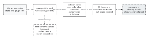
A quasiparticle projection requires a narrow, resolved spectral structure and slow central variation, with width and gradients assigned a common counting. Off-shell tails, overlapping peaks, or leading coherence invalidate scalar shell kinetics even if a nominal pole can be fitted. The microscopic-matching step may use cuts only for a controlled weak-coupling quasiparticle kernel; the dashed branch retains matrix-valued transport rather than forcing coherence into a scalar $f$. The diagram is schematic and not to scale.

The sections Spectral shell and width, Joint gradient counting, and Gauge and basis dependence provide the text and equation equivalent of the shell box and coherence branch.

A retained-term table

Suppose $\Gamma/E\sim\epsilon$, $\partial_X/E\sim\epsilon$, and branch separations are $O(E)$. Then shell shifts from $\operatorname{Re}\Sigma_R$, first gradients, and collision terms can all enter at $O(\epsilon)$, depending on coupling counting. A term proportional to $\partial_X/\Gamma$ is $O(1)$ rather than $O(\epsilon^2)$ and must be resummed. The explicit scaling of masses, occupation amplitudes, and infrared momenta must accompany this table; there is no universal assignment valid in every regime.

As a check, integrate $\mathcal A$ against a smooth test function $h(p^0)$. If $h$ varies on scale $\Lambda_h$, the delta-shell error is controlled parametrically by the resolved width over $\Lambda_h$. If $h$ contains a second nearly coincident shell or a sharp threshold, $\Lambda_h$ is small and the expansion fails even though $\Gamma/E\ll1$.

Gauge and basis dependence

Pole locations of physical excitations can be gauge independent under suitable conditions, while residues, off-shell spectral shapes, and truncated damping rates can retain gauge dependence. A consistent calculation includes the vertex corrections required by Ward identities at the same order. In mixing systems, an $X$-dependent diagonal basis creates connection terms of order $\partial_X/\Delta E$; dropping them precisely when levels approach degeneracy loses coherent transitions.

The validation map pairs each leading assumption with a diagnostic. The four columns are independent: each dashed vertical arrow names a failure mode and points to a corresponding test, without allowing one passed test to substitute for another.

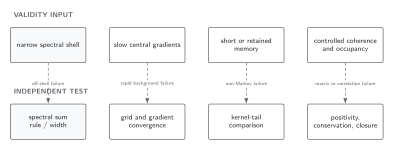
A resolved narrow shell and slow central variation are independent leading requirements. Their paired tests are spectral normalization and width control, plus convergence under grid and gradient-order refinement. The remaining memory and coherence columns must also pass before a scalar kinetic claim is accepted. The absence of horizontal arrows is deliberate: no column supplies or licenses another. The diagram is schematic and not to scale.

The sections Spectral shell and width, Joint gradient counting, and A retained-term table provide the text and equation equivalent, including numerical tests, of the first two columns.

Failure tests

• Resolve the full spectral function and vary the fit window before declaring a shell.
• Compare $\Gamma$ with energy, branch gaps, background frequencies, and collision thresholds.
• Evaluate the first omitted Moyal term and finite-memory correction.
• Keep widths until all potentially singular shell products are integrated.
• Test pole and collision quantities under gauge and scale variation at common order.
• Near critical, infrared, or degenerate regimes, switch to stochastic, matrix, or full two-time dynamics rather than extrapolating scalar kinetics.

Exercise

Why can the limit $\Gamma\to0$ make a Markov approximation worse?

Solution

The spectral peak becomes sharper, improving an on-shell projection, but its relative-time correlator decays on the longer scale $\Gamma^{-1}$. If the distribution changes on a fixed time $\tau_X$, the memory parameter $1/(\Gamma\tau_X)$ grows. Shell control and memory control are distinct limits.

Continue

Build processes at the retained order on collision kernels and test every ratio in kinetic validity and breakdown.

References

• Arnold, P., Moore, G. D., and Yaffe, L. G. (2003). “Effective Kinetic Theory for High Temperature Gauge Theories.” Journal of High Energy Physics 2003(01), 030. arXiv:hep-ph/0209353; DOI.
• Weldon, H. A. (1983). “Simple Rules for Discontinuities in Finite-Temperature Field Theory.” Physical Review D 28, 2007–2015. DOI.