Multiplicative, Colored, and Conserved Noise

Multiplicative, colored, non-Gaussian, and conserved noise are different extensions. Multiplicative noise requires a stochastic prescription and noise-induced drift; colored noise introduces memory and can often be made Markovian only by enlarging the state; conserved noise has derivative covariance and an exact zero mode; non-Gaussian noise requires higher cumulants in the response functional.

Required background. Use the MSRJD functional and detailed balance and FDT.

Helpful background. Non-Markovian memory kernels develops controlled memory representations.

Multiplicative noise and stochastic calculus

For one variable, the midpoint prescription introduced by Stratonovich 1966, §§ 2–3 writes

$$dx=a_S(x)\,dt+b(x)\circ dW$$

in the Stratonovich convention is equivalent to the Itô equation

$$dx=a_I(x)\,dt+b(x)\,dW, \qquad a_I=a_S+\frac12b\,b'.$$

The correction follows from $\langle dW^2\rangle=dt$. Other noise normalizations change the factor. Therefore the written pair $(a,b)$ does not define a process until the convention is named.

The Itô Fokker–Planck current is

$$J=a_IP-\frac12\partial_x(b^2P).$$

If a target equilibrium density $P_{\mathrm{eq}}\propto e^{-\mathcal F/T}$ is specified, setting $J=0$ determines the required drift. Omitting the derivative of $b^2$ changes the stationary measure. In MSRJD form the same correction appears through the determinant and equal-time response prescription.

Colored noise as an enlarged Markov process

An Ornstein–Uhlenbeck colored force can be defined by

$$\tau_\xi\dot\xi=-\xi+\sqrt{2D}\,\eta(t), \qquad \langle\eta(t)\eta(t')\rangle=\delta(t-t').$$

Its stationary covariance is

$$\langle\xi(t)\xi(t')\rangle =\frac{D}{\tau_\xi}e^{-|t-t'|/\tau_\xi}.$$

As $\tau_\xi\to0$, this tends distributionally to $2D\delta(t-t')$. The pair $(x,\xi)$ is Markovian even though $x$ alone has memory. Expanding in $\tau_\xi/\tau_x$ is controlled only when the slow variable changes little over the noise correlation time and no resonant frequency probes $1/\tau_\xi$.

Equilibrium colored noise generally requires a matching friction kernel through a generalized FDT. Adding colored forcing to local friction creates a driven nonequilibrium model unless that relation is satisfied.

Conserved noise

Model B for a conserved scalar is

$$\partial_t\phi =\Gamma\nabla^2\frac{\delta\mathcal F}{\delta\phi} +\nabla\cdot\boldsymbol\zeta,$$

with

$$\langle\zeta_i(t,\mathbf x)\zeta_j(t',\mathbf x')\rangle =2\Gamma T\,\delta_{ij}\delta(t-t') \delta^{(d)}(\mathbf x-\mathbf x').$$

Integrating over space with periodic or no-flux boundaries gives $d\int\phi/dt=0$ for every realization. In Fourier space the scalar noise power is proportional to $k^2$, so the $k=0$ mode receives no forcing. Adding ordinary white scalar noise would violate conservation.

The first arrow in the schematic carries more information than the word “noise”: multiplicative noise requires a stochastic prescription, colored noise requires memory or auxiliary variables, and conserved noise requires the corresponding derivative structure and boundary conditions.

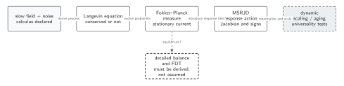
Multiplicative, colored, and conserved noises modify different parts of the process and cannot be exchanged as stylistic choices. The Fokker–Planck operator and MSRJD action must be rederived from the stated calculus and enlarged state space. Detailed balance and FDT require a matched drift, diffusion, and mobility structure; they do not follow from Gaussianity or stationarity alone. The diagram is schematic and not to scale.

The sections Multiplicative noise and stochastic calculus, Colored noise as an enlarged Markov process, and Conserved noise give the text and equation equivalent of the declared-process and probability-evolution boxes.

Non-Gaussian noise and closure

If the eliminated force has connected cumulants beyond the covariance, integrating it produces response-field vertices $\tilde\phi^n$ with $n>2$. Replacing it by Gaussian noise is a central-limit or coarse-graining approximation whose scale and tails must be tested. Rare events and multiplicative couplings can keep higher cumulants relevant.

Use the stochastic and kinetic closure validity table for convention, spectrum, regulator, positivity, stationarity, and white-noise-limit checks.

Failure tests

• Translate Itô and Stratonovich forms and recover identical observables.
• Measure the full noise spectrum and higher cumulants.
• Take the colored-to-white limit at fixed integrated covariance.
• Verify the matching friction kernel for equilibrium claims.
• Test exact conservation realization by realization.
• Vary ultraviolet cutoff; multiplicative white noise can generate regulator-sensitive drift.
• Include the first omitted non-Gaussian cumulant.

Exercise

For $b(x)=\sigma x$, what Itô drift corresponds to Stratonovich drift $a_S=-\gamma x$?

Solution

$b b'/2=(\sigma x)(\sigma)/2=\sigma^2x/2$. Hence $a_I=(-\gamma+\sigma^2/2)x$. Using $-\gamma x$ in both conventions would define two different processes.

Continue

Use the conserved or nonconserved slow-variable content on dynamic universality classes and test its nonequilibrium consequences on quenches and aging.

References

• Fox, R. F. (1986). “Functional-Calculus Approach to Stochastic Differential Equations.” Physical Review A 33, 467–476. DOI.
• Itô, K. (1944). “Stochastic Integral.” Proceedings of the Imperial Academy 20, 519–524. DOI.
• Stratonovich, R. L. (1966). “A New Representation for Stochastic Integrals and Equations.” SIAM Journal on Control 4, 362–371. DOI.