Moment Hierarchies and Closure Schemes

Moments of a kinetic equation form an exact infinite hierarchy. A fluid theory appears only after a matching prescription and a closure for the omitted moments. That closure must be counted in Knudsen number and departure from equilibrium, preserve the licensed conserved quantities, and produce a hyperbolic, stable system over its claimed regime.

Required background. Use collision kernels and distribution moments.

Helpful background. Linearized relaxation modes identifies slow moment combinations, while Israel–Stewart transient theory develops causal relativistic closures.

Exact hierarchy

Multiply the kinetic equation by basis functions $\psi_A(p)$ and integrate:

$$M_A(x)=\int dP\,\psi_A(p)f(x,p), \qquad \partial_\mu M_A^\mu =\int dP\,\psi_A C[f]+\text{force terms}.$$

If $\psi_A$ is a collision invariant, the right-hand side vanishes after summing species. Otherwise its evolution contains higher moments because streaming raises tensor rank. Density couples to current, current to stress, stress to third moments, and so on.

Decompose near local equilibrium,

$$f=f_{\mathrm{eq}}(T,\mu,u^\mu)+\delta f.$$

Matching conditions define $T,\mu,u^\mu$ by requiring selected moments of $\delta f$ to vanish. Landau matching sets the energy flow in the local rest frame to zero; other frames impose different conditions. Transport coefficients and transient fields are frame dependent even when observables are not.

Grad and Chapman–Enskog closures

A Grad-type closure, introduced in Grad 1949, §§ 3–5, expands $\delta f$ in a finite polynomial basis,

$$\delta f=f_{\mathrm{eq}}(1+\eta f_{\mathrm{eq}}) \left[a+b_\mu p^\mu+c_{\mu\nu}p^\mu p^\nu+\cdots\right],$$

and determines coefficients from retained moments. Truncation can make $f$ negative at large momentum because a polynomial eventually dominates the equilibrium tail.

Chapman–Enskog instead solves the kinetic equation iteratively in gradients. At first order it yields Navier–Stokes constitutive relations; at higher order, naive gradient truncations can be acausal or unstable. Transient closures promote dissipative moments to independent variables, for example

$$\tau_\pi\Delta^{\mu\nu}_{\alpha\beta}D\pi^{\alpha\beta} +\pi^{\mu\nu} =2\eta\sigma^{\mu\nu}+\text{second-order couplings}.$$

$\tau_\pi$ is tied to nonhydrodynamic relaxation, not chosen merely to repair causality. Hyperbolicity and stability constrain the complete coefficient set and background state.

The final box of the hierarchy is a warning as much as an endpoint: taking moments creates an exact infinite hierarchy, while closing it introduces a model whose omitted moments and regime of validity must remain visible.

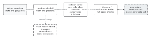
Moment equations are exact projections of a licensed kinetic equation, but any finite Grad, Chapman–Enskog, or relaxation closure adds ordering and positivity assumptions. Conservation fixes selected low moments without bounding every omitted mode. The upstream microscopic-matching step can use cuts for controlled weak-coupling quasiparticle kernels. Matrix-valued coherent transport is an alternative reduction when internal-state coherence is leading, not a scalar moment closure appended at the end. The diagram is schematic and not to scale.

The sections Exact hierarchy, Grad and Chapman–Enskog closures, and Closure obligations provide the text and equation equivalent of the final closure box and its retained error.

Checked relaxation closure

For a homogeneous shear moment in a linear collision model,

$$\partial_t\pi^{ij}=-\frac{1}{\tau_\pi}\pi^{ij}+2\eta\sigma^{ij}/\tau_\pi,$$

a constant applied shear gives

$$\pi^{ij}(t)=2\eta\sigma^{ij} +[\pi^{ij}(0)-2\eta\sigma^{ij}]e^{-t/\tau_\pi}.$$

The solution approaches Navier–Stokes after the nonhydrodynamic transient. It checks the sign and normalization but not the value of $\tau_\pi$: that must follow from the parent collision operator or matching data.

Closure obligations

The relevant small parameters are the Knudsen number $\mathrm{Kn}=\ell_{\mathrm{mfp}}/L$ and inverse Reynolds numbers measuring dissipative stresses relative to equilibrium scales. A formal gradient order is not enough when coefficients are large, moments have heavy tails, or a collision eigenvalue becomes small.

The shared stochastic and kinetic closure table records the moment basis, matching, closure order, positivity, convergence, and parent-equation comparison.

The final column of the validation map prevents a closure from inheriting credibility merely because the upstream kinetic equation passed shell and gradient tests. Positivity, conservation, closure sensitivity, and numerical resolution remain separate requirements.

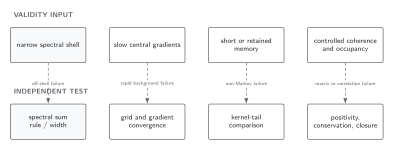
A finite moment system is acceptable only if its retained variables capture the slow sector and its predictions are stable under closure enlargement. Conservation of selected moments does not guarantee positivity or small omitted moments. The upper and lower rows list assumptions and diagnostics in four independent columns; each dashed vertical arrow pairs a failure mode with a relevant test. The diagram is schematic and not to scale.

The sections Exact hierarchy, Grad and Chapman–Enskog closures, and Closure obligations give the text and equation equivalent of the closure column and its failure modes.

Failure tests

• Increase the moment basis and compare target observables.
• Compare Grad and Chapman–Enskog closures under matched inputs.
• Monitor $f\ge0$ and fermionic $f\le1$ rather than only moment values.
• Verify exact collision invariants before and after closure.
• Test characteristic speeds, hyperbolicity, and linear stability across the claimed state range.
• Vary $\mathrm{Kn}$ and inverse Reynolds numbers independently.
• Benchmark the finite system against the parent kinetic solution.

Exercise

Why does exact conservation of the first few moments not establish accuracy of a moment closure?

Solution

Collision invariants are protected algebraically, so many different closures can conserve them. They can still predict different stresses, heat fluxes, tails, and transient modes. Accuracy requires convergence with basis size or comparison with the parent distribution, in addition to conservation.

Continue

Use linearized collision modes to choose slow moments and validity and breakdown to test the resulting closure.

References

• Grad, H. (1949). “On the Kinetic Theory of Rarefied Gases.” Communications on Pure and Applied Mathematics 2, 331–407. DOI.
• Israel, W., and Stewart, J. M. (1979). “Transient Relativistic Thermodynamics and Kinetic Theory.” Annals of Physics 118, 341–372. DOI.