Lines of Constant Physics and Continuum Extrapolation

A controlled continuum result is a joint inference over a tuned line of constant physics, scale and operator renormalization, finite-volume corrections, and the cutoff expansion allowed by the regulator symmetries. The fit must preserve correlations among axes and ordinates, compare plausible artifact models, identify an asymptotic window, and survive held-out tests such as removing the coarsest or finest spacing. Three spacings and a small $\chi^2$ do not suffice if the trajectory drifts or the model is unidentifiable.

Required background. Scale Setting and Dimensionless Ratios supplies shared scale covariance. Lattice Perturbation Theory, Symanzik Analysis, and Improvement supplies the allowed cutoff powers. Bare Parameters, Tuning Conditions, and Continuum Targets defines the target trajectory.

Helpful background. Regulator Removal and Renormalized Predictions gives the general continuum and scheme logic. Nonperturbative Renormalization, Mixing, and Step Scaling is needed when the observable carries a nontrivial operator scheme.

In the chapter’s observable-chain table, this page combines the preceding controls into the improvement-and-continuum and reported-quantity stages.

Executing a line of constant physics

Let $R_\alpha$ be the renormalized tuning quantities and $R_\alpha^\star$ their target values. At each spacing, measured ensembles rarely land exactly on the target. Write residuals

\delta R_{\alpha e}=R_{\alpha e}-R_\alpha^\star

for ensemble $e$ . A dimensionless target observable $Q_e$ can be expanded locally as

Q_e^{\mathrm{tuned}} =Q_e^{\mathrm{meas}} -\sum_\alpha J_{\alpha e}\delta R_{\alpha e} +O(\delta R^2), \qquad J_{\alpha e}=\frac{\partial Q}{\partial R_\alpha}.

The slopes $J_{\alpha e}$ must be constrained by nearby ensembles, reweighting, or a justified response model. Setting residuals to zero in the table while leaving $Q$ unchanged hides mistuning rather than correcting it.

The rest of this page uses a raw-data convention: $Q_e^{\mathrm{meas}}$ remains the fitted ordinate, so the mistuning response appears with a plus sign in the model below. An equivalent pre-corrected analysis would fit $Q_e^{\mathrm{tuned}}$ and omit the response term; applying both operations would double count the correction.

Continuum-fit conventions. The page fits dimensionless renormalized observables and uses the site-wide conventions. The constant-physics conditions, reference scale, operator scheme and $\mu$ , volume prescription, mass trajectory, cutoff variable, improvement status, and fit covariance are local. A common continuum value across regulators is imposed only after matching the same target observable.

When $Q$ , the scale $X$ , and tuning ratios share configurations, they form one joint data vector. Paired bootstrap or jackknife samples can carry their covariance through interpolation, renormalization, and the final fit. If stages are performed separately, use a joint nuisance-parameter likelihood rather than attaching independent errors afterward.

A dimensionless continuum model

Choose $x_e=a_eX_e$ , where $X$ is a fixed physical reference. For an $O(a)$ -improved bulk observable with leading $a^2$ effects, a representative model is

Q_e^{\mathrm{meas}} =Q_0 +c_2x_e^2 +c_{2\ell}x_e^2\log x_e +c_4x_e^4 +d_LF(m_eL_e) +\sum_\alpha J_\alpha\delta R_{\alpha e} +\epsilon_e +O(\delta R^2).

Here $\epsilon_e$ is the correlated residual described by the joint statistical model. Replacing $J_{\alpha e}$ by one $J_\alpha$ assumes the response is approximately constant over the local tuning neighborhood, so its variation changes $Q$ only beyond the retained linear order. Check that approximation with the same nearby ensembles or reweighting used to determine the slope; otherwise retain ensemble-dependent $J_{\alpha e}$ or add a controlled response expansion.

Not every term should be included automatically. The Symanzik basis, anomalous dimensions, boundary conditions, and improvement status determine which powers and logarithms are plausible. $F(mL)$ comes from the finite-volume regime: an exponential form is justified only with a mass gap and short-range interactions; massless or long-range theories can have power-law effects.

$x_e$ is measured, not exact. Because it shares the reference $X_e$ with $Q_e$ , ordinary least squares on central $x_e$ values can bias slopes and understate uncertainty. A joint model treats the true scales as latent quantities constrained by their measurements, or repeats the entire fit on paired resamples. This is an errors-in-variables problem; Kelly 2007, §§III–IV gives an explicit likelihood treatment allowing heteroscedastic and correlated measurement errors.

The simplest useful set of competing models might be:

\begin{array}{ll} M_1:& Q_0+c_2x^2,\\ M_2:& Q_0+c_2x^2+c_4x^4,\\ M_3:& Q_0+c_2x^2+c_{2\ell}x^2\log x,\\ M_4:& Q_0+c_4x^4 \quad\text{for a claimed $O(a^2)$ cancellation}. \end{array}

A linear candidate is not identifiable if its weighted design matrix lacks full column rank; a very large condition number or nearly singular parameter covariance signals the practical version of the same problem. In a prior-regularized fit, report whether the likelihood or the prior supplies each constraint. Residual structure and held-out predictions then test the specified model. For a probabilistic synthetic fixture, “coverage” is a repeated-replica property—the stated fraction of intervals must contain the injected value—not something established by one noiseless solve. Averaging poorly identified models can hide rather than quantify ignorance.

Finding the asymptotic window

The Symanzik expansion is asymptotic in $a\Lambda\ll1$ ; its effective-action basis and improvement logic are developed in Symanzik 1983, Part I, pp. 187–204 and applied perturbatively in Symanzik 1983, Part II, pp. 205–227. Coarse points can have small statistical errors and dominate a fit while lying outside that regime. Diagnose the window through:

successive removal of the coarsest spacing;
stability of $Q_0$ and leading coefficients;
dimensionless residuals plotted against $x^2$ , $mL$ , and tuning residuals;
consistency of the predicted power in held-out observables; and
agreement of two regulator families with different artifact coefficients.

Removing the finest point tests the opposite failure: a result apparently determined by one high-leverage ensemble. Leave-one-spacing-out predictions should reproduce each omitted point within the declared model and covariance. To make this an assessment rather than a new round of model selection, fix the candidate terms and prior rules without consulting the omitted point; this follows the distinction between cross-validatory choice and assessment in Stone 1974, pp. 111–133.

The “finest-only” fit is not automatically safer. If it contains too little lever arm to determine $c_2$ , its continuum intercept becomes prior dominated. Report the information content or parameter correlations, not only the central value.

Separate finite-volume, mass, and cutoff limits

The cleanest design includes a volume study at one or more spacings so the $L$ dependence is constrained independently of $a$ . If only one volume exists at each spacing and $mL$ changes monotonically with $a$ , cutoff and volume slopes are confounded.

A possible massive-theory target is

Q_\infty =\lim_{L\to\infty} \left[ \lim_{a\to0}^{R_\alpha=R_\alpha^\star} Q_R(a,L) \right].

A chiral or critical limit adds another axis whose order can matter. For spontaneous symmetry breaking, the infinite-volume limit generally precedes removal of an explicit symmetry-breaking mass. Writing a joint fit does not prove the limits commute; it merely parameterizes one chosen trajectory.

Finite-volume amplitude extraction is a different problem: discrete spectra are the input to a quantization condition, not nuisance corrections to be extrapolated away. Continue to Finite Volume as a Controlled Deformation for that regime.

Cross-regulator universality test

Suppose two matched actions $A$ and $B$ have the same target but different leading coefficients:

Q_A(a)=Q_0+c_Aa^p+\cdots, \qquad Q_B(a)=Q_0+c_Ba^q+\cdots.

A joint fit with common $Q_0$ and action-specific artifacts tests continuum agreement. Forcing the common intercept by construction is meaningful only if separate fits are also compatible and the observable, renormalization scheme, physical volume, and tuning conditions truly match.

Agreement is not independent if both actions use the same operator matching, scale input, finite-volume model, and analysis code. State the shared sources of uncertainty. A structurally distinct Hamiltonian or other formulation can provide stronger evidence once its own continuum program is complete.

A synthetic multi-spacing example

Let $x_i=(0.30,0.22,0.16,0.11)$ and $\ell_j=(4,6)$ . Their Cartesian product defines eight noiseless means

Q_{ij}^{\mathrm{mean}} =1.20+0.50x_i^2+0.30e^{-\ell_j}.

The design row is $X_{ij}=(1,x_i^2,e^{-\ell_j})$ , so the formula specifies every input to the deterministic linear-algebra check. It should recover the injected coefficient vector $(Q_0,c_2,d_L)=(1.20,0.50,0.30)$ to the solver tolerance. No statistical coverage claim follows from this noiseless fixture. A replica study must additionally publish its random-number algorithm and seed, the covariance of the measured $Q$ , $x$ , and any shared scale nuisance, and the interval construction being tested.

Three injected failures are especially useful:

retain only $mL=4$ , which makes the finite-volume column proportional to the intercept and therefore confounds $Q_0$ with the volume shift;
omit the coarsest point until the $a^4$ model becomes unconstrained but apparently precise under a narrow prior;
shift the tuning ratio by an amount correlated with $a^2$ and omit the response term.

A pipeline should flag each through residuals, rank or prior sensitivity, and a failed held-out prediction.

The QFT.org 2026 Chapter 2 benchmark, validated snapshot constructs the eight rows directly and recovers $(1.2000000000,0.5000000000,0.3000000000)$ . The full design has rank $3$ and normalized condition number $4.37$ . Keeping only $mL=4$ reduces the rank to $2$ because the intercept and finite-volume columns are proportional; locking $mL$ to a function of $(aX)^2$ leaves full rank but raises the normalized condition number to $100.56$ . These deterministic checks diagnose rank and conditioning, not statistical coverage.

Avoiding double counting

An uncertainty source enters once at the stage where its stochastic or epistemic model is defined. Examples of double counting include:

propagating scale uncertainty through $Q$ and then adding the same scale error again in physical units;
applying a finite-volume correction with uncertain coefficient and also taking the full corrected–uncorrected shift as an independent error;
averaging artifact models and adding their full spread a second time;
including renormalization factors in paired resamples and again as independent Gaussian errors; or
treating mistuning corrections as both nuisance parameters and post-fit systematic shifts.

Construct a dependency graph or joint variable list before fitting so every shared input has one source and all downstream correlations are visible.

The map below is the chapter’s full closure test. Follow the path from tuned bare parameters to the final dimensionless observable and verify that scale, matching, mixing, finite volume, cutoff fitting, and every held-out comparison remain distinct correlated inputs.

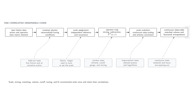
A lattice action, measure, operators, and symmetries define a line of constant physics and regulator-consistent calculation, which meets a named continuum scheme in operator matching; a direct route or optional step-scaling detour rejoins before correlated volume and continuum analysis, while four failure exits reject invalid claims. — A continuum prediction requires a tuned bare trajectory, a regulator-consistent calculation, and a renormalized observable in a named scheme. When momentum-space lattice perturbation theory is used, its propagators, vertices, and Brillouin zone must be retained unless a controlled matching or subtraction justifies a continuum replacement. Step scaling or scheme conversion is optional when the matching scale is already suitable. The failure exits reject an untuned trajectory, an unjustified continuum propagator inside a lattice loop, a defining input counted as a prediction, and a one-spacing or unsupported extrapolation. Schematic, not to scale.

Observable-level validation checklist

Before accepting a continuum result, require:

declared renormalized constant-physics conditions and measured residuals at every spacing;
scale, operator-renormalization, and target data propagated jointly;
independent variation of volume and cutoff for the claimed finite-volume model;
artifact powers and logarithms justified by exact regulator symmetries and improvement status;
at least three useful spacings within an identified asymptotic window, with enough lever arm to constrain the leading term;
coarsest-point, finest-point, and leave-one-spacing-out tests;
competing identifiable fit models and transparent prior sensitivity;
residual plots against every independent error axis;
a second action or formulation when universality is material; and
one non-double-counted uncertainty decomposition reconstructing the total covariance.

Exercises

1. Confounded design. Suppose all ensembles satisfy $mL=4+10(aX)^2$ . Explain why a fit $Q=Q_0+c(aX)^2+d e^{-mL}$ may not identify $c$ and $d$ well.

Solution

Both regressors become deterministic functions of the same $aX$ sequence and can be highly collinear over a short range. Their coefficients can trade off while leaving predictions nearly unchanged. Add multiple volumes at fixed spacing or impose independently validated finite-volume information.

2. Shared continuum intercept. Derive the normal-equation structure for two action families with a common $Q_0$ and separate slopes $c_A,c_B$ . What comparison tests whether the common-intercept constraint is reasonable?

Solution

Let $y$ collect both action families, let $C$ be their full covariance, and set $\beta=(Q_0,c_A,c_B)^{\mathsf T}$ . The design rows are $(1,a^p,0)$ for action $A$ and $(1,0,a^q)$ for action $B$ . Generalized least squares obeys

\left(X^{\mathsf T}C^{-1}X\right)\widehat\beta =X^{\mathsf T}C^{-1}y, \qquad \operatorname{Cov}(\widehat\beta) =\left(X^{\mathsf T}C^{-1}X\right)^{-1},

when $C$ is treated as known and $X$ as fixed. For the separate-intercept comparison, use $\beta_{\mathrm{sep}}=(Q_{0,A},Q_{0,B},c_A,c_B)^{\mathsf T}$ , with rows $(1,0,a^p,0)$ for $A$ and $(0,1,0,a^q)$ for $B$ . If $h=(1,-1,0,0)^{\mathsf T}$ , then

\widehat\Delta_0=h^{\mathsf T}\widehat\beta_{\mathrm{sep}}, \qquad \operatorname{Var}(\widehat\Delta_0) =h^{\mathsf T}\operatorname{Cov}(\widehat\beta_{\mathrm{sep}})h.

Compare the common-intercept fit with this separately estimated $\Delta_0=Q_{0,A}-Q_{0,B}$ and its uncertainty. Compatibility, rather than the imposed equality alone, supports a shared limit.

What you can now do

You should now be able to design a correlated multi-spacing extrapolation that preserves constant physics, scale and matching covariance, finite-volume control, and plausible Symanzik alternatives. You should also be able to reject a smooth fit whose asymptotic window, identifiability, or uncertainty structure is unsupported. The resulting continuum observable is ready for interpretation by the relevant physics volume, not automatically evidence that the full regulator family defines a mathematically constructed QFT.

References

Kelly, Brandon C. “Some Aspects of Measurement Error in Linear Regression of Astronomical Data.” The Astrophysical Journal 665, no. 2 (2007): 1489–1506. doi:10.1086/519947.
OpenAI Codex for QFT.org. “Lattice Observables and Continuum Inference Benchmark.” JavaScript source, validated 25 August 2026. SHA-256 d76924d8c724cb7c9307fb38265336495fa3ff1a98103b3fa4fa734262647c2a. Reproducibility record.
Stone, M. “Cross-Validatory Choice and Assessment of Statistical Predictions.” Journal of the Royal Statistical Society: Series B (Methodological) 36, no. 2 (1974): 111–133. doi:10.1111/j.2517-6161.1974.tb00994.x.
Symanzik, Kurt. “Continuum Limit and Improved Action in Lattice Theories. I. Principles and $\phi^4$ Theory.” Nuclear Physics B 226, no. 1 (1983): 187–204. doi:10.1016/0550-3213(83)90468-6.
Symanzik, Kurt. “Continuum Limit and Improved Action in Lattice Theories. II. O( $N$ ) Nonlinear Sigma Model in Perturbation Theory.” Nuclear Physics B 226, no. 1 (1983): 205–227. doi:10.1016/0550-3213(83)90469-8.