Complete Lattice Error Budgets

A complete lattice error budget connects every material source to an estimator, propagation rule, correlation structure, validation test, and residual limitation. The total is not obtained by naming many percentages: categories can overlap, distributions can be asymmetric, and some uncontrolled effects impose a limit on the claim rather than a quantifiable standard deviation.

Required background. Equilibration and chain diagnostics establish the realized ensemble; multi-stage uncertainty propagation carries correlations; and continuum extrapolation defines spacing and volume inference.

Helpful background. Blinding and independent reproduction control analysis-choice feedback.

Components of a claim-level budget

Local error-budget convention and regime. The budget applies to one named observable, regulator sequence, analysis version, and claim. Components are classified by physical or statistical source rather than organizational stage; correlated probabilistic sources are propagated jointly, bounded nonprobabilistic effects remain bounds, and an unidentified effect is a stop condition rather than an invented standard deviation. The final wording cannot exceed the weakest validated component.

The table below is the chapter’s common inference and reproducibility record.

Source	Estimator or bound	Correlation and propagation	Validation	Residual risk or stop
Finite sampling	autocorrelation-aware covariance or replicas	aligned blocks across all observables	AR(1), exact, or repeated-chain coverage	slow tail unresolved
Equilibration and sectors	start/cut comparisons, sector histories	common to every quantity on affected streams	independent starts and regeneration	no equilibrium sector coverage
Stochastic or solver noise	nested repeats, residual sequence	conditional within configurations	exact solves or dense small system	tolerance-induced bias
Spectral and fit inference	window/model alternatives, residual model	joint time/channel covariance	synthetic closure and holdout	target state not identifiable
Scale and tuning	shared nuisance distribution	common across ensembles and dimensions	ratio closure or alternative input	circular tuning
Operator matching	$Z$ matrix, subtraction, scheme/window variations	shared gauge and matching data	Ward identity, step scaling, scheme conversion	power divergence uncontrolled
Finite volume	theory-informed sequence or bound	correlated with fitted masses and scale	second volume and branch assumptions	long-range formula invalid
Cutoff and continuum	several spacings and alternative powers/actions	global covariance	omit coarsest point; alternative regulator	intercept not identified
Analysis choice	frozen alternatives or calibrated selection	correlated across stages	blind and independent analysis	adaptation not represented
External inputs	published covariance or bounded range	retain common provenance	update and unit closure	source covariance unavailable

Every row names a failure condition. If it occurs, enlarging an unrelated statistical error does not repair the scientific gap.

Autocorrelation-aware finite-sampling estimates and their window dependence are treated by Wolff 2004, pp. 143–153, while slow lattice-QCD modes and conservative tail control are analyzed by Schaefer, Sommer, and Virotta 2011, pp. 93–119. The distinction between a probabilistic error and a bounded or procedural systematic is discussed by Barlow 2002, lecture article.

Combining components

When sources can be represented by a joint approximately Gaussian nuisance vector $\boldsymbol\eta$ with covariance $C_\eta$, propagate through the full analysis. For a linearized final result,

$$\sigma_Q^2=\mathbf g^TC_\eta\mathbf g, \qquad g_i=\frac{\partial Q}{\partial\eta_i}.$$

Quadrature is the special case of zero off-diagonal covariance. Linear addition is a worst-case bound only for specified signs and ranges; it is not a generic “conservative” combination.

For discrete model alternatives or asymmetric extrapolations, report a mixture, envelope, or separate directional interval whose meaning is stated. If a source is bounded but not probabilistic, keep it as a bound rather than converting it to a Gaussian standard deviation by convention.

The dependency graph shows where double counting most often enters.

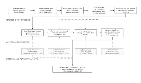
The final uncertainty inherits serial dependence, shared inputs, fit choices, matching, and continuum inference. Coverage and independent checks test the whole pipeline; they are not interchangeable with internal stability. The diagram is schematic.

Precision and wording follow the weakest component

A result with $0.2\%$ statistical error but an untested $3\%$ continuum model is not a sub-percent continuum determination. A result from a single frozen topological sector is not an equilibrium topological observable, even if local quantities are stable. A matrix element with uncontrolled power-divergent mixing is not repaired by precise bare correlators.

Useful claim labels include:

• finite-ensemble estimate at stated regulator;
• renormalized finite-spacing result;
• volume-corrected result within a specified range expansion;
• continuum-trending result under listed fit families;
• continuum-extrapolated result with a stated residual bound.

Keep methodological limitations in the prose beside the result. Do not compress a nonidentifiability or missing limit into an anonymous “systematic.”

End-to-end validation

Test more than each component in isolation:

1. generate synthetic histories with known autocorrelation and a known multistage target;
2. inject burn-in, late drift, covariance rank loss, an extra spectral state, and a shared-scale shift;
3. run the exact production selection, resampling, fit, matching, and continuum pipeline;
4. measure bias and interval coverage over repetitions;
5. verify that each named adversary either fails a gate or enlarges the correct component;
6. reproduce one result with independent code and one with an alternative regulator or observable.

Coverage in a synthetic family does not prove the physical model, but failed coverage disproves the uncertainty procedure for that family.

Adversarial failure: a quantified total hides an unidentified limit

Suppose a finite-spacing observable has independently validated statistical, scale, and matching uncertainties of $0.2\%$, $0.3\%$, and $0.4\%$. Their uncorrelated quadrature is

$$\sqrt{0.2^2+0.3^2+0.4^2}\%=0.54\%.$$

If only one lattice spacing exists, however, the continuum correction is unidentified. Quoting a “continuum result” with $0.54\%$ total uncertainty is invalid even when every included component has perfect synthetic coverage. The correct response is to report a finite-spacing result with those quantified components and make the continuum limit a stop condition until additional spacings or a defensible bound exist.

Observable-level validation checklist

• Name the exact observable, regulator sequence, analysis version, and claim to which the budget applies.
• For every material source, record an estimator or bound, propagation rule, correlations, validation result, and residual risk or stop condition.
• Trace shared scale, tuning, matching, fit, and continuum inputs through the dependency graph and test explicitly for duplication or omission.
• Run the production pipeline on repeated synthetic histories with injected burn-in, long tails, covariance loss, omitted states, and shared-input shifts; report bias and interval coverage.
• Reproduce the target with an independent analysis and, where the claim requires it, an alternative regulator, volume, or observable.
• Apply the unidentified-continuum adversary above and verify that the claim wording stops at finite spacing rather than absorbing the missing limit into an arbitrary percentage.

Common pitfalls

Choosing categories by organizational stage. The same scale input can enter tuning, matching, and continuum conversion. Classify by source and dependency, not by which team handled it.

Adding all alternative shifts in quadrature. Alternatives can be correlated views of one missing term. Use a coherent candidate set or covariance model.

Reporting a total without component definitions. A reader must be able to reconstruct what varied, how it propagated, and which risks remain unquantified.

Learning outcomes

1. Given a lattice result, construct a non-double-counted error table that records source, estimator or bound, propagation, correlation, validation, and residual risk for every material uncertainty.
2. Given a numerically small total containing an injected unidentified component, set the precision and scientific wording by the weakest controlled element and reject a claim that exceeds it.

Exercises

1. Two components have standard deviations $2$ and $3$ with correlation $-1/2$. Find the combined standard deviation for their sum.

Solution

$\sigma^2=2^2+3^2+2(-1/2)(2)(3)=7$, so $\sigma=\sqrt7\simeq2.65$, not $\sqrt{13}$.

2. How should an unbounded, unidentified continuum effect be entered in the table?

Solution

As a stop condition that limits the claim to finite spacing or continuum trending. Assigning an arbitrary percentage would falsely imply quantification.

References

• Barlow, R. (2002). Systematic errors: facts and fictions. In Advanced Statistical Techniques in Particle Physics. arXiv.
• Schaefer, S., Sommer, R., and Virotta, F. (2011). Critical slowing down and error analysis in lattice QCD simulations. Nuclear Physics B, 845, 93–119. DOI.
• Wolff, U. (2004). Monte Carlo errors with less errors. Computer Physics Communications, 156, 143–153. DOI.