PEPS and Higher-Dimensional Field Theories

A PEPS extends the virtual-bond construction to two or more spatial dimensions, but its finite bond dimension and its contraction approximation are independent controls. The state is well defined once its local tensors are fixed; expectation values generally require an approximate environment, so a computed “variational energy” is an upper bound only when the contraction error is itself bounded tightly enough.

Required background. Entanglement structure and tensor-network ansätze supplies the graph, virtual-bond, gauge, and Schmidt-truncation grammar.

Helpful background. Lattice gauge Hamiltonians and Gauss’s law supplies physical gauge sectors for gauge-theory PEPS.

Projected entangled pairs and their environments

On a square lattice, attach a virtual space of dimension $\chi$ to each end of every edge, prepare a maximally entangled virtual pair on each edge, and map the four incident virtual spaces to the physical local space with $P_x$:

$$|\Psi(A)\rangle =\bigotimes_x P_x \bigotimes_{\langle xy\rangle}|\omega_\chi\rangle_{xy}, \qquad |\omega_\chi\rangle=\sum_{\alpha=1}^{\chi}|\alpha\alpha\rangle.$$

In components, $P_x$ is the local PEPS tensor $A^{s_x}_{\ell r u d}$. The higher-dimensional variational construction was introduced by Verstraete and Cirac 2004. The virtual bonds give an area-compatible bound on Schmidt rank, but do not establish that a fixed $\chi$ approximates a chosen continuum state to a stated tolerance. Exact contraction of general two-dimensional PEPS is computationally hard; this is a structural limitation, not merely a software choice Schuch et al. 2007.

The norm is a two-dimensional double-layer network. Contracting physical indices produces a local transfer tensor

$$E_{(\ell\ell')(rr')(uu')(dd')} =\sum_s A^s_{\ell r u d}(A^s_{\ell'r'u'd'})^*.$$

Boundary MPS, corner transfer matrices, tensor renormalization, or related constructions approximate the infinite environment of $E$. A concrete infinite-size PEPS algorithm based on repeated environment contraction is given by Jordan et al. 2008. Denote the environment control collectively by $\chi_{\rm env}$. It is not the PEPS bond dimension $\chi$: increasing $\chi$ enlarges the state family and usually makes the environment harder to resolve.

Regulator and convention box. Specify spatial dimension and lattice, unit cell, boundary conditions, physical dimension $d_{\rm loc}$, PEPS bond dimensions, exact symmetry sectors, contraction family, all environment dimensions and stopping rules, optimizer and initialization, $L$, $a$, and operator normalization. For an infinite PEPS, “thermodynamic limit” refers to the chosen environment fixed point; it does not remove finite-$\chi$ or finite-$\chi_{\rm env}$ effects.

The network geometry and the continuum gate are shown below. Inspect the PEPS label and the separate approximate-environment control.

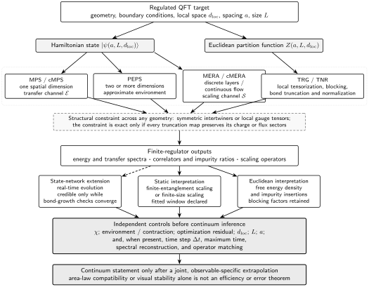
PEPS represents a Hamiltonian state, while its two-dimensional norm and observables require a contraction procedure. The schematic map makes the PEPS bond dimension and environment contraction distinct before any continuum interpretation.

Exactly contractible copy-tensor fixture

On four sites, define a tensor network whose virtual bit is copied to every physical leg. Contracting the internal copy indices gives

$$|\Psi_{\rm copy}\rangle =\frac{|0000\rangle+|1111\rangle}{\sqrt2}.$$

This is a finite PEPS with virtual dimension $\chi=2$. Direct enumeration gives

$$\langle\Psi_{\rm copy}|\Psi_{\rm copy}\rangle=1, \qquad \langle Z_iZ_j\rangle=1, \qquad \langle X_i\rangle=0, \qquad \langle X_1X_2X_3X_4\rangle=1.$$

It tests index orientation, double-layer normalization, long-range sector structure, and impurity insertion. A contraction that returns $\langle X_i\rangle\neq0$ has mixed the two virtual sectors or selected an unintended boundary fixed point. This benchmark is deliberately non-injective; it prevents an implementation from assuming a unique transfer fixed point everywhere.

Variational optimization with an approximate objective

For the exact normalized PEPS state,

$$E[A]=\frac{\langle\Psi(A)|H|\Psi(A)\rangle} {\langle\Psi(A)|\Psi(A)\rangle}\geq E_0.$$

But an approximate environment produces $\widetilde E[A;\chi_{\rm env}]$. Unless $|\widetilde E-E|$ is bounded, $\widetilde E$ need not remain above $E_0$, and optimizing it may favor tensors that exploit contraction bias. The repair is not simply a tighter optimizer tolerance. Re-evaluate frozen tensors with increasing $\chi_{\rm env}$ and at least one structurally different contraction, then reoptimize after the environment is demonstrably adequate.

Simple, full, gradient, and variational updates differ in which environment information they retain. Their method names are not accuracy certificates. The PEPS construction, transfer structure, and contraction distinction are reviewed by Cirac et al. 2021, §§ III and VI.

The joint control map makes the coupling between $\chi$ and $\chi_{\rm env}$ explicit. Follow its fixed-tensor contraction scan before interpreting an optimizer plateau.

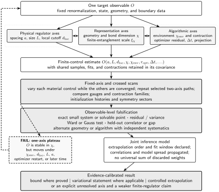
For PEPS, ansatz, environment, contraction, and optimization errors are correlated but not interchangeable. The diagram is schematic: credible evidence includes frozen-tensor re-contraction, reoptimization, physical-regulator scans, and held-out observables.

QFT continuum and gauge structure

A higher-dimensional QFT calculation adds three regulators that a spin-model PEPS discussion can leave hidden: a bosonic or link local cutoff $d_{\rm loc}$, the lattice spacing $a$, and operator matching. At each $a$, tune the bare Hamiltonian on a line of constant physics and test

$$R(a,L,d_{\rm loc},\chi,\chi_{\rm env}) =R_*+c_a a^p+c_L e^{-mL}+\delta_{\rm loc}+\delta_\chi+\delta_{\rm env}+\cdots,$$

without treating the displayed terms as statistically independent by default. Gauge invariance may be imposed through intertwiner tensors, but truncating the represented flux set can still distort dynamics while preserving Gauss’s law exactly. The construction is treated on Symmetric and Gauge-Invariant Tensor Networks.

Use the chapter’s tensor-network regulator and error record to report the geometry, environment, observable, and capability boundary.

Higher-dimensional implementations must retain the frozen-tensor environment tests above; dated reach and comparative performance remain conditional on the Research dossier.

Adversarial failure: an energy below the exact ground state

An optimizer reports an energy slightly below an exact small-lattice $E_0$ and the value is stable with additional sweeps. This is not superior variational performance; it falsifies the evaluated quotient or its claimed error. Freeze the tensor and enlarge $\chi_{\rm env}$, compare boundary-MPS and corner methods, verify norm positivity and Hermiticity, and only then resume optimization. Sweep stability probes the approximate objective, not the exact PEPS energy.

Observable-level validation checklist

• Contract a product state and the copy-tensor fixture exactly.
• Freeze tensors and scan every environment dimension before reoptimization.
• Compare at least two contraction geometries or algorithms at selected points.
• Report norm, Hermiticity, energy variance or local residual, and initialization history.
• Check exact global or gauge constraints and boundary sectors.
• Vary $d_{\rm loc}$, $L$, and $a$ independently of $\chi$ and $\chi_{\rm env}$.
• Match the operator and validate a held-out correlator, ratio, or small-volume spectrum.
• State finite-PEPS evidence separately from any continuum claim; dated reach belongs in the Research methods dossier.

What you should be able to do

After this page, you should be able to:

1. specify a higher-dimensional PEPS calculation with separate state-bond, environment, local-space, volume, and spacing controls; and
2. design frozen-tensor and reoptimization tests that distinguish ansatz, optimizer, contraction, symmetry, and continuum failures.

Exercises

1. Variational status. An approximate contraction gives $\widetilde E=-1.002$ for a Hamiltonian whose exact finite-volume ground energy is $-1$. What can be concluded?

Solution

Only that the approximate evaluation error is at least consequential at the quoted precision. The exact energy of the normalized PEPS still obeys $E[A]\geq-1$, but $\widetilde E$ is not a certified upper bound. Freeze $A$ and converge or bound the contraction before making a variational claim.

2. Independent axes. Why is a sequence $(\chi,\chi_{\rm env})=(2,16),(3,36),(4,64)$ insufficient to identify the separate errors?

Solution

Both controls change together, so a drift or plateau can result from cancellation. Add fixed-$\chi$ environment scans and fixed-contraction-quality bond scans; selected crossed points estimate their interaction.

References

• Cirac, J. Ignacio, David Pérez-García, Norbert Schuch, and Frank Verstraete. “Matrix Product States and Projected Entangled Pair States: Concepts, Symmetries, Theorems.” Reviews of Modern Physics 93 (2021): 045003. DOI.
• Jordan, Jacob, Román Orús, Guifré Vidal, Frank Verstraete, and J. Ignacio Cirac. “Classical Simulation of Infinite-Size Quantum Lattice Systems in Two Spatial Dimensions.” Physical Review Letters 101 (2008): 250602. DOI.
• Schuch, Norbert, Michael M. Wolf, Frank Verstraete, and J. Ignacio Cirac. “Computational Complexity of Projected Entangled Pair States.” Physical Review Letters 98 (2007): 140506. DOI.
• Verstraete, Frank, and J. Ignacio Cirac. “Renormalization Algorithms for Quantum-Many Body Systems in Two and Higher Dimensions.” arXiv:cond-mat/0407066 (2004). arXiv.