Cross-Method Validation and Reliability Standards

A finite-density method is reliable only over the region where its correctness conditions, exact or sign-free benchmarks, overlap, and regulator scaling have all been demonstrated for the target observable. Cross-method agreement strengthens a result when the methods have genuinely different failure mechanisms. Agreement outside either method’s validated domain—or agreement produced by a shared truncation, ensemble, or normalization—does not raise the claim ceiling.

Required background. Anatomy and severity of a sign problem supplies phase and overlap metrics. Complex Langevin correctness supplies stochastic boundary tests. Dual, worldline, and tensor reformulations supplies exact-transformation tests.

Helpful background. Reweighting, Taylor expansion, and imaginary density, Lefschetz thimbles and holomorphic flow, and canonical, fugacity, and density-of-states methods supply the remaining method-specific contracts.

A method-neutral reliability ladder

Convention and regulator card. A validation domain is a set of lattice spacings, volumes, temperatures, chemical potentials, masses, observables, and algorithm settings for which every named diagnostic passes. “Agreement” means compatible estimates of the same normalized observable at the same regulator, with correlated uncertainties and shared inputs accounted for. Dated capability assessments remain Research claims.

Use the following ladder in order.

1. Algebraic identity: prove the reweighting, dual, contour, stochastic, or Fourier relation at finite regulator, including Jacobians and boundary sectors.
2. Exact microfixture: reproduce a finite integral or enumerated small lattice and at least one phase-sensitive observable.
3. Negative control: move to a point or deliberately broken implementation where the characteristic failure must be detected.
4. Sign-free overlap: compare with direct importance sampling at imaginary $μ$, opposite-flavor chemical potentials, or another exactly positive regime.
5. Method overlap: compare two methods with different correctness assumptions inside both demonstrated domains.
6. Scaling: repeat over volume, lattice spacing, truncation, arithmetic precision, and algorithmic parameters.
7. Claim boundary: state the largest connected domain supported by the preceding evidence; do not interpolate through an unvalidated gap.

The first four steps test correctness; the fifth tests transport across methods; the sixth tests physical inference. Passing a later-looking visual comparison cannot substitute for an earlier algebraic or negative-control failure.

Finite-density method reliability matrix

The table records the minimum evidence needed for each route. “Research” in the final column is a claim ceiling for reach beyond exact or sign-free fixtures, not a judgment that the underlying identity is speculative.

Method and target	Severity and overlap evidence	Correctness conditions and tunables	Exact fixture and failure witness	Cost, residual uncertainty, evidence ceiling
Phase or multiparameter reweighting: normalized real-$μ$ observables	Average phase, joint log-weight tails, numerator–denominator covariance, proposal support	Exact weight ratio; common support; reference point and path varied	One-angle Bessel result; clipped weights or a deliberately missed rare sector must fail	Effective independent samples and tail sensitivity versus volume; controlled only inside measured overlap
Taylor expansion at $μ=0$	Coefficient covariance, order stability, complex-zero or ratio diagnostics	Symmetry-complete derivatives; expansion order and resummation varied	Exact fixture coefficients; injected nearby complex zero must limit reach	Stochastic derivative cost plus truncation; claim stops before demonstrated analytic boundary
Imaginary-$μ$ continuation	Withheld imaginary points, fit leverage, common analytic interval	Exact periodicity and symmetry; ansatz, range, and order varied	$\cos\mu_I\to\cosh\mu$ fixture; alternative analytic functions matching training points expose extrapolation ambiguity	Continuation-model and discretization uncertainty; Research beyond overlap with Taylor or reweighting
Exact dual, worldline, bag, or tensor variables	Residual sign, sector occupancy, winding autocorrelation, cutoff tails	Invertible algebraic map; all constraints, sectors, Jacobians, observable defects; integer or bond cutoff varied	Small-lattice enumeration; omit one winding or charge sector as failure witness	Transformation, contraction, mixing, and truncation cost; model-specific ceiling, never a generic cure
Complex Langevin: holomorphic observables	Drift and excursion tails, determinant-zero distance, mode occupancy	Vanishing boundary terms, adequate holomorphy, ergodicity, zero-step limit; cooling/stabilization varied	Exact one-angle density; stationary trajectory near a drift pole must be rejected	Autocorrelation, tail resolution, step and stabilization bias; current extrapolative reach is Research
Thimbles or holomorphic flow: deformed-contour observables	Residual phase, Jacobian tails, mode transitions, sector weights	Same homology, no singular crossing, complete thimbles, exact Jacobian; flow time varied	Flow-time-invariant fixture; omitted contributing saddle or trapped mode must fail	Jacobian, multimodal, residual-phase, and Stokes uncertainty; large-volume reach is Research
Canonical, fugacity, or density of states: sector and reconstructed observables	Coefficient dynamic range, transform condition number, sector/tail support	Correct Fourier period, relative normalization, full required sectors or bounded tails; grid, precision, binning varied	Exact three-mode fixture and convolution; undersampled Fourier grid must alias	Precision and tail amplification versus volume and fugacity; real-density reach is Research until cross-checked

The table’s claim boundaries follow the explicit worst-case qualifiers of Troyer and Wiese 2005, the drift-decay correctness condition of Nagata, Nishimura, and Shimasaki 2016, and the canonical projection of Hasenfratz and Toussaint 1992. These sources establish identities and conditional results; they do not establish a current universal winner.

Why agreement can be misleading

Suppose two estimates of the same scalar observable are

$$y_1=\theta+b_s+b_1+\epsilon_1, \qquad y_2=\theta+b_s+b_2+\epsilon_2,$$

where $b_s$ is a shared bias, $b_i$ are method-specific biases, and $ε_i$ are statistical errors. Their difference is

$$y_1-y_2=(b_1-b_2)+(\epsilon_1-\epsilon_2),$$

so agreement cancels $b_s$ completely. Examples include the same coarse gauge ensemble, the same scale setting, the same omitted charge sectors, the same imaginary-density fit ansatz, or the same incorrect observable normalization.

Combination is justified only after bias controls. With an estimated covariance matrix $C$ for unbiased measurements, the best linear unbiased combination is

$$\hat\theta=\frac{\mathbf1^TC^{-1}y}{\mathbf1^TC^{-1}\mathbf1}, \qquad \operatorname{Var}(\hat\theta)=(\mathbf1^TC^{-1}\mathbf1)^{-1}.$$

This formula does not absorb unknown method bias. If diagnostics leave bounded biases $|b_i|\le B_i$, propagate them separately or use a conservative envelope. Do not inflate or shrink statistical errors until disagreeing central values overlap.

The common exact campaign

Use

$$Z_1(\mu)=2\pi[(1+h^2)I_0(\beta_0)+2hI_1(\beta_0)\cosh\mu]$$

at $\beta_0=1$, $h=0.2$, real $\mu=0,0.5,1,1.5$, imaginary $\mu_I=0,\pi/4,\pi/2,3\pi/4$, and independent-copy volumes $V=1,4,16,64$. The campaign carries three observables:

$$f_V=-\frac1V\log Z_V, \qquad n_V=\frac1V\partial_\mu\log Z_V, \qquad \chi_V=\frac1V\partial_\mu^2\log Z_V.$$

For independent copies these equal the one-copy intensive values, while phase severity and canonical dynamic range scale strongly with $V$. That separation makes the fixture valuable: a method cannot excuse a drifting intensive observable as new many-body physics.

Run direct quadrature, reweighting, Taylor expansion, imaginary-axis Fourier projection, canonical convolution, complex Langevin, and finite holomorphic flow where implemented. Each method must return its own diagnostics, not only $f_V,n_V,\chi_V$. The toy fixture tests code paths and failure detection; it does not validate continuum QCD.

Disagreement and claim ceilings

When methods disagree:

1. freeze the target definition and all shared inputs;
2. determine whether the point lies inside each validation domain;
3. rerun exact and negative controls at matched numerical precision;
4. expose method-specific latent variables—weights, sectors, drift tails, modes, coefficients—not merely final observables;
5. vary one tunable at a time and preserve correlations;
6. leave the discrepancy unresolved if no diagnostic identifies it.

Do not average incompatible estimates. A disagreement outside one method’s domain downgrades that method at the point; a disagreement inside both domains indicates at least one correctness assessment is incomplete. Either case lowers, rather than widens, the physical claim.

A minimal ceiling language is:

• Exact at finite regulator: algebraic identity plus enumeration or exact quadrature.
• Validated numerical window: all correctness diagnostics and independent comparisons pass on a bounded domain.
• Controlled physical inference: volume, continuum, and truncation limits are included in one uncertainty statement.
• Research indication: evidence is promising but at least one correctness, scaling, or independence requirement remains open.

Adversarial failure cases

Two methods share the same configurations. Correlated statistical agreement is presented as independent confirmation. Estimate cross-covariance and add a genuinely independent ensemble or exact calculation.

Validation only at the easiest point. A method matches at $μ=0$ and is extrapolated through a region where its phase, drift, or condition number changes exponentially. Validate along the entire path and stop at the first failed diagnostic.

Only positive controls. Every tuned method fits the fixture after choices are selected. Freeze choices, test a hostile point, and require the method to flag its own failure without seeing the exact answer.

Continuum agreement at one volume. Discretization trends agree, but finite-volume effects differ between methods. Perform matched two-dimensional scaling or bound the missing direction.

The severity map supplies the common diagnostic language for the comparison table. A method must state whether it changes phase variance, target overlap, representation cost, or only the asymptotic problem family; improvement on one axis cannot be reported as a universal cure.

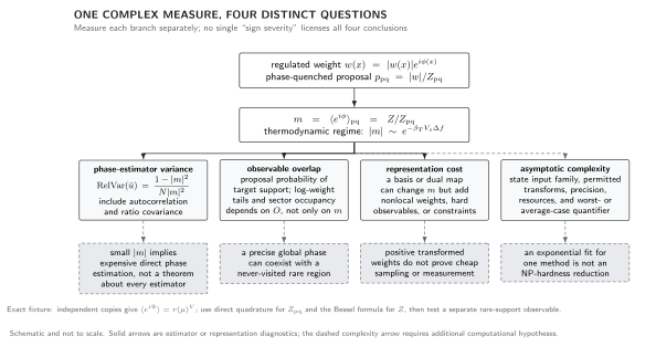
The sign problem has distinct diagnostics. The average phase fixes direct phase-estimator signal-to-noise and may scale as $e^{-\beta_TV_s\Delta f}$; overlap depends on the target observable and proposal measure; a variable change can trade phase for nonlocality or hard observables; and worst-case complexity requires a separately specified problem family. The map is schematic, not a quantitative performance comparison.

The correctness map complements the severity map by assigning a falsifier to each method family. Agreement enters the common gate only after its own overlap, exact-duality, stochastic-boundary, contour-homology, or reconstruction-precision condition has passed.

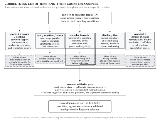
Each reformulation has a different correctness condition and a characteristic counterexample. Apparent numerical convergence is insufficient when overlap is absent, a dual sector or Jacobian is missing, complex-Langevin boundary terms survive, a contributing thimble is omitted, or canonical and density-of-states cancellations exceed resolved precision. The map is schematic and does not rank current algorithms.

Observable-level validation checklist

• Fix the observable, charge normalization, action, volume, lattice spacing, and physical parameters before comparison.
• Record which inputs and configurations are shared; include cross-method covariance.
• Require an algebraic check, exact fixture, negative control, sign-free overlap, and method-overlap point.
• Track phase, overlap, drift, thimble, sector, tail, and condition diagnostics appropriate to each method.
• Vary volume, lattice spacing, truncation, precision, and algorithm settings in the same parameter region.
• State the demonstrated domain and the first failed or missing criterion; classify any extension as Research evidence.

Exercises

1. Shared bias

Two methods give $y_1=1.02\pm0.03$ and $y_2=1.01\pm0.03$, but both omit a correction known only to satisfy $0\le b_s\le0.10$. What does their agreement establish?

Solution

The difference constrains method-specific effects and statistical fluctuation, but it contains no information about $b_s$. A combined estimate may reduce statistical variance, yet the shared systematic interval remains. The result cannot be quoted with a total uncertainty near $0.02$ until the common correction is computed or bounded more tightly.

2. A negative-control decision

A complex-Langevin run matches the exact density at $μ=0.5$ and $1$, but at $1.5$ has a power-law drift tail and disagrees by five standard deviations. A thimble run agrees at all three points but has no transitions between two known modes at $1.5$. Set the claim boundary.

Solution

Complex Langevin is validated only through the largest connected region before its tail criterion fails; it cannot support the $μ=1.5$ point. The thimble central value at $1.5$ is also not validated because missing mode mixing leaves its relative normalization uncontrolled. Cross-method evidence supports the overlap region through $μ=1$; the $μ=1.5$ value remains Research evidence despite one correct-looking number.

Learning outcomes

After working this page, you should be able to:

• Build and execute a method-specific reliability matrix for one observable, including exact, negative, sign-free, overlap, and scaling tests.
• Detect shared-assumption agreement, propagate cross-method covariance and residual bias separately, and set a claim boundary at the first unsupported point.

Handoff

The chapter’s Euclidean inference methods end here. Hamiltonian lattice field theory develops transfer matrices, Hilbert-space regulators, spectra, and real-time dynamics; comparisons across formulations must still match the same regulator, observable, and limit.

References

• Hasenfratz, Anna, and David Toussaint. “Canonical Ensembles and Nonzero Density Quantum Chromodynamics.” Nuclear Physics B 371 (1992): 539–549. doi:10.1016/0550-3213(92)90247-9.
• Nagata, Keitaro, Jun Nishimura, and Shinji Shimasaki. “Argument for Justification of the Complex Langevin Method and the Condition for Correct Convergence.” Physical Review D 94 (2016): 114515. doi:10.1103/PhysRevD.94.114515.
• Troyer, Matthias, and Uwe-Jens Wiese. “Computational Complexity and Fundamental Limitations to Fermionic Quantum Monte Carlo Simulations.” Physical Review Letters 94 (2005): 170201. doi:10.1103/PhysRevLett.94.170201.