Encoding Fields and Truncating Local Hilbert Spaces

An encoding is scientifically adequate when it maps the regulated Hamiltonian, state sector, and observable into simulator degrees of freedom while exposing locality overhead and a separately convergent local-Hilbert error. Bosonic fields require an energy- or amplitude-controlled truncation; fermionic maps trade anticommutation for strings or auxiliary structure; gauge-link encodings must say which group algebra and representations remain exact. Qubit count alone certifies none of these properties.

Required background. What counts as a quantum simulation of QFT? supplies the target-to-observable contract. Local Hilbert-space regulators, quantum links, and finite gauge groups supplies the regulator physics. Hilbert-space truncation as a regulator supplies projector and omitted-state reasoning.

Helpful background. Fock space, vacuum, and particle number supplies occupation-basis conventions.

Local encodings and what they preserve

Convention and regulator card. Work at fixed spatial lattice spacing $a$, finite volume $L^d$, and finite energy window $E\le E_*$. The local encoding is an isometry $V_x:P_x\mathcal H_x\to(\mathbb C^2)^{\otimes n_x}$ or to a qudit/CV subspace. The projector $P_x$ and convergence sequence must be stated. Errors are evaluated on a declared many-body sector, not by an impossible uniform approximation to an unbounded operator.

For a scalar site, one useful field-grid encoding chooses $d_{\rm loc}=2^{n_q}$ values

$$\phi_j=-\phi_{\max}+j\Delta_\phi, \qquad \Delta_\phi=\frac{2\phi_{\max}}{d_{\rm loc}},$$

and obtains the conjugate grid through a discrete Fourier transform. Two tails must be controlled independently:

$$\epsilon_{\rm amp}=\langle\psi|\mathbf1_{|\phi|>\phi_{\max}}|\psi\rangle, \qquad \epsilon_{\rm mom}=\langle\psi|\mathbf1_{|\pi|>\pi_{\max}}|\psi\rangle.$$

Increasing $\phi_{\max}$ at fixed $d_{\rm loc}$ reduces amplitude clipping but coarsens $\Delta_\phi$ and lowers the Fourier momentum range. The two parameters therefore require a joint convergence study. For localized low-energy scalar states, sampling theory can make digitization error decrease rapidly after both tails are resolved, but that result is state- and Hamiltonian-dependent Klco and Savage 2019, §§ II–IV.

An occupation encoding instead retains $|0\rangle,\ldots,|n_{\max}\rangle$. Unary encoding uses $O(n_{\max})$ qubits and local ladder operations; binary encoding uses $\lceil\log_2(n_{\max}+1)\rceil$ qubits but generally compiles ladder operators into longer controlled arithmetic. Neither resource statement is complete without gate synthesis and state support.

No finite-dimensional pair obeys the canonical commutator exactly: $\operatorname{Tr}[\widetilde\phi,\widetilde\pi]=0$ whereas $\operatorname{Tr}(i\mathbf1)=i d_{\rm loc}$. The correct statement is a low-energy matrix-element test such as

$$\epsilon_{\rm CCR}(E_*)= \left\|P_{E_*}\bigl([\widetilde\phi,\widetilde\pi]-i\mathbf1\bigr)P_{E_*}\right\|.$$

Calling the truncated algebra “canonical” without this qualification hides a mathematical obstruction.

Fermions and gauge links

For an ordered set of fermionic modes, the Jordan–Wigner map

$$c_j=\left(\prod_{k<j}Z_k\right)\frac{X_j+iY_j}{2}$$

preserves the canonical anticommutation relations exactly on the encoded Fock space. Its parity string can make geometrically local hopping nonlocal in more than one spatial dimension. Alternative parity encodings redistribute this overhead; they do not remove the need to count compiled support, ancillas, and constraints.

For a compact gauge link, a representation cutoff keeps irreducible representations up to a stated label, a quantum-link construction replaces the link algebra by a finite representation, and a finite-group encoding replaces the continuous group itself. These are different regulated theories at finite cutoff. A useful convergence record tests plaquette or electric energies, the group multiplication law that remains exact, Gauss generators, and at least one observable as the representation set grows. Discrete-subgroup digitization can require an improved action to reach the intended scaling regime; the existence of a compact binary encoding is not enough Alexandru et al. 2019.

Continuous-variable and analog encodings avoid a qubit field grid only if their accessible quadratures and interactions match the regulated variables over the populated energy window. One must still bound finite squeezing, nonlinearities, mode leakage, calibration uncertainty, and unwanted couplings. Platform realization requires its own calibration evidence.

The flow through the encoding link

In the shared end-to-end map, inspect the first two solid arrows: both the Hamiltonian and the observable must cross the encoding, and the constraint test must act on the encoded state rather than only on ideal basis labels.

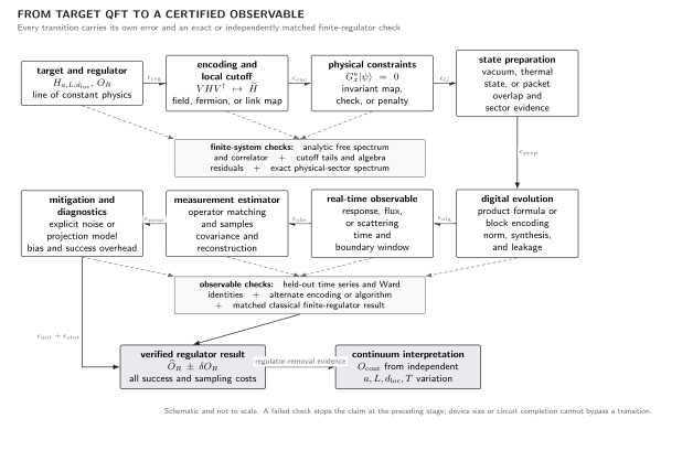
Encoding is one transition in an end-to-end calculation. Its required outputs are encoded Hamiltonian, state, observable, and physical-sector action; its checks are local-cutoff convergence, algebra residuals, exact small-system spectra, and observable agreement. Later circuit execution cannot compensate for a failed map. The diagram is schematic and platform independent.

The chapter-wide minimum claim–resource–evidence record requires the encoding and its convergence test to be named in every claim tier.

Analytic benchmark: one harmonic mode

For $H=(\pi^2+\omega^2\phi^2)/2$, the exact ground-state density is

$$|\psi_0(\phi)|^2=\sqrt{\frac{\omega}{\pi}}e^{-\omega\phi^2}.$$

The amplitude-tail probability of a symmetric field window is

$$\epsilon_{\rm amp}=\operatorname{erfc}(\sqrt\omega\,\phi_{\max}).$$

Choose $\phi_{\max}$ from this analytic tolerance, then increase $d_{\rm loc}$ until the discrete Fourier kinetic energy, the first excitation gap, and $\langle\phi^2\rangle=1/(2\omega)$ converge. For a free periodic chain, repeat mode by mode against

$$\omega_k^2=m_0^2+4a^{-2}\sin^2(ka/2).$$

This test separates amplitude clipping, grid aliasing, and spatial-lattice dispersion. Turning on $\lambda\phi^4$ only after the free tests pass gives a clean interacting benchmark.

Adversarial failures

One cutoff direction. Increasing $d_{\rm loc}$ while fixing an inadequate $\phi_{\max}$ can produce a stable but clipped spectrum. Vary the window and resolution independently.

Exact Hamiltonian, approximate observable. A compact encoding reproduces low energies, but the measured field operator is projected or wrapped incorrectly. Held-out matrix elements and correlators must converge, not just eigenvalues.

Broken algebra outside the training states. A variationally prepared state has small energy but support near the truncation boundary, where commutators fail. Measure boundary occupation and algebra residuals on the evolved state.

Local qubit count as locality. A binary code uses few qubits per site while compiled hopping contains long parity or arithmetic strings. Count the actual operator support and synthesis error.

Observable-level validation checklist

• Specify the projector or grid, field range, local dimension, ordering, boundary convention, and exact encoded sector.
• Test both Hamiltonian and observable matrix elements on a low-energy reference subspace.
• Vary amplitude or occupation cutoff separately from grid resolution and spatial lattice spacing.
• Measure truncation-boundary occupation, commutator or group-algebra residuals, and constraint leakage during evolution.
• Compare exact diagonalization of a small interacting system and the analytic free-chain dispersion.
• Report encoded qubits or qudits together with operator support, ancillas, synthesis cost, calibration uncertainty, and convergence evidence.

Exercises

1. Why a finite canonical pair is impossible

Prove that finite matrices $Q$ and $P$ cannot satisfy $[Q,P]=i\mathbf1$.

Solution

Cyclicity gives $\operatorname{Tr}[Q,P]=\operatorname{Tr}(QP)-\operatorname{Tr}(PQ)=0$. But $\operatorname{Tr}(i\mathbf1)=id_{\rm loc}\ne0$. Therefore the relation can hold only approximately on a proper subspace, or a different finite algebra must be used.

2. Choose a field window

For a unit-frequency oscillator, choose $\phi_{\max}$ so that the exact ground-state probability outside the window is below $10^{-6}$.

Solution

Solve $\operatorname{erfc}(\phi_{\max})<10^{-6}$. Since $\operatorname{erfc}^{-1}(10^{-6})\simeq3.459$, any $\phi_{\max}>3.459$ suffices. Grid resolution must still be checked independently.

Learning outcomes

After working this page, you should be able to:

• Map a regulated scalar, fermion, or compact-gauge Hamiltonian and observable to qubits or qudits, and state the resulting local-dimension, locality, ancilla, and synthesis overhead.
• Design a convergence campaign that separates field-window or occupation error, grid aliasing, algebra or constraint error, and spatial-regulator error using an exact low-energy reference sector.

Handoff

Enforcing gauge symmetry and constraints turns an encoded gauge-link space into a controlled physical sector. Digital Hamiltonian simulation and algorithmic error converts the resulting terms into an evolution algorithm. Device-level analog or CV calibration remains a separate implementation task.

References

• Alexandru, Andrei, Paulo F. Bedaque, Siddhartha Harmalkar, Henry Lamm, Scott Lawrence, and Neill C. Warrington. “Gluon Field Digitization for Quantum Computers.” Physical Review D 100 (2019): 114501. doi:10.1103/PhysRevD.100.114501.
• Klco, Natalie, and Martin J. Savage. “Digitization of Scalar Fields for Quantum Computing.” Physical Review A 99 (2019): 052335. doi:10.1103/PhysRevA.99.052335.