Digital Hamiltonian Simulation and Algorithmic Error

Digital Hamiltonian simulation approximates $e^{-iHt}$ from encoded primitives. Its guarantee is meaningful only after the Hamiltonian decomposition, operator norms, commutator structure, oracle or block-encoding costs, gate synthesis, symmetry action, and target observable tolerance are fixed. Query complexity and compiled gate complexity are different quantities, and an asymptotic bound is not an implementation certificate.

Required background. Encoding fields and truncating local Hilbert spaces supplies the finite encoded terms and their support. Commutators and operator exponentials supplies Baker–Campbell–Hausdorff control.

Helpful background. Real-time evolution, scattering, and observable extraction supplies the regulator-level target dynamics.

Product formulas and commutator error

Convention and regulator card. Fix a finite encoded Hilbert space and write $H=\sum_{j=1}^{M}H_j$, with each $H_j$ Hermitian and its implementation specified. Simulation time $t$ is physical, $r$ is the number of steps, and $\delta=t/r$. Operator-norm bounds apply to the whole encoded space unless an explicitly justified invariant subspace is stated. Encoding, state, noise, and measurement errors are not included in $\epsilon_{\rm alg}$.

The first-order Lie product formula is

$$S_1(\delta)=e^{-iH_1\delta}\cdots e^{-iH_M\delta}, \qquad U_1(t)=S_1(t/r)^r.$$

For $H=A+B$, Baker–Campbell–Hausdorff gives

$$e^{-iA\delta}e^{-iB\delta} =\exp\left[-i(A+B)\delta-\frac{\delta^2}{2}[A,B] +O(\delta^3)\right].$$

Thus the global leading error scales as $t^2\|[A,B]\|/r$, with constants and higher nested commutators fixed by the chosen bound. The key point is commutator scaling: replacing it by $\|A\|\|B\|$ can badly overestimate local lattice problems, while ignoring it can miss a volume dependence. Modern product-formula bounds organize the error through nested commutators and locality Childs et al. 2021, Theorems 10–12.

The symmetric second-order step

$$S_2(\delta)=e^{-iA\delta/2}e^{-iB\delta}e^{-iA\delta/2}$$

cancels the quadratic local term and has global $O(t^3/r^2)$ error under finite nested-commutator bounds. Higher-order or randomized formulas change the commutator sum, number of exponentials, and synthesis pattern; they should be compared at the same observable error and total compiled cost.

Block encodings and query guarantees

Suppose a unitary $U_H$ block-encodes $H/\alpha$:

$$(\langle0|\otimes I)U_H(|0\rangle\otimes I)=H/\alpha, \qquad \alpha\ge\|H\|.$$

Qubitization and quantum signal processing can approximate $e^{-iHt}$ using a number of block-encoding queries scaling as $O(\alpha t+\log(1/\epsilon_{\rm alg}))$ under their stated access model Low and Chuang 2019. This is a query statement. A resource record must additionally construct state-preparation/select oracles, count ancillas, decompose each query into the target logical gate set, and include synthesis precision and success amplification.

For local QFT Hamiltonians, $\alpha$ and oracle cost can depend on spatial volume, lattice spacing, coupling, and local dimension. Comparing $O(\alpha t)$ queries with a product formula’s exponential count without compiling either side is not a performance comparison.

Error allocation and symmetry-preserving compilation

For a bounded observable $O$, it is often wasteful to demand a global unitary error far below the final experimental tolerance. A sufficient bound is

$$|\langle O\rangle_{\widetilde U}-\langle O\rangle_U| \le2\|O\|\,\|\widetilde U-U\|,$$

but a state- or observable-specific bound may be tighter. Allocate a target $\epsilon_O$ among

$$\epsilon_O\ge \epsilon_{\rm reg}+\epsilon_{\rm enc}+\epsilon_{\rm prep} +\epsilon_{\rm formula}+\epsilon_{\rm synth} +\epsilon_{\rm noise}+\epsilon_{\rm meas}.$$

The allocation is a design variable: decreasing Trotter error after sampling or local-truncation error dominates only increases cost.

If every compiled primitive commutes with a represented Gauss generator $G_x^a$, the product formula preserves the sector exactly even at finite step. If only the sum $H$ commutes while individual $H_j$ do not, Trotterization can leak at finite $\delta$. The compiler must therefore report symmetry commutators for its actual term grouping.

Algorithmic error in the shared flow

The figure locates digital evolution between prepared state and measurement. Inspect the distinction between an operator-norm transition check and the later observable-level test.

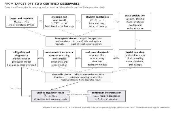
Digital Hamiltonian simulation is one controlled arrow, not the whole QFT calculation. Product-formula or block-encoding error, logical synthesis, physical-sector preservation, and an exact finite-system time series are separate checks. The schematic diagram does not compare algorithm or hardware performance.

The minimum claim–resource–evidence record requires algorithm, norm, symbolic cost, and matched finite-regulator check to remain in the same row.

Analytic benchmark: two noncommuting terms

Take $A=\omega X/2$ and $B=gZ/2$. Since

$$[A,B]=-\frac{i\omega g}{2}Y,$$

one first-order step has leading norm error $|\omega g|\delta^2/4$, and $r$ steps give the estimate

$$\epsilon_1(t,r)\simeq\frac{|\omega g|t^2}{4r}$$

when higher terms are small. Exact exponentiation of $H=(\omega X+gZ)/2$ provides an independent answer: the Bloch vector rotates about $(\omega,0,g)$ with frequency $\Omega=\sqrt{\omega^2+g^2}$. A benchmark should verify the predicted $r^{-1}$ and $r^{-2}$ slopes for first- and second-order formulas, then inject a small symmetry-breaking term to confirm the leakage diagnostic responds.

For the chapter’s free scalar chain, the same campaign compares every measured mode frequency with $\omega_k^2=m_0^2+4a^{-2}\sin^2(ka/2)$ while varying only the formula step. This is the prescribed regulator-level benchmark; hardware execution is not part of this page.

Adversarial failures

Norm bound with an unconstructed oracle. A qubitization query count is quoted, but loading coefficients costs exponentially many gates. The access model, data structure, and compiled oracle cost must be explicit.

Step convergence toward the wrong encoded Hamiltonian. $\delta\to0$ removes formula error but leaves field digitization and omitted operators unchanged. Compare with an exact matrix built from the intended regulator, not only with a finer circuit.

Symmetry of the sum only. $[H,G]=0$ while $[H_j,G]\ne0$. A coarse product formula can populate unphysical sectors even though the exact unitary does not.

Favorable error cancellation. One time and one observable happen to cancel Trotter and synthesis errors. Test several times, noncommuting observables, and both signs or orderings of the step.

Observable-level validation checklist

• Give the term decomposition, support, coefficient norms, commutator or block-encoding normalization, and access model.
• State the algorithm, order, step count or query count, ancillas, logical primitives, and synthesis tolerance.
• Verify symmetry commutators for the compiled terms and measure physical-sector leakage.
• Reproduce exact small-system time series and the predicted convergence order over a resolved range.
• Allocate the final observable tolerance across encoding, preparation, algorithm, synthesis, noise, and sampling before optimizing.
• Report query and compiled logical-gate costs separately, with all state-loading and success-amplification overheads.

Exercises

1. Step count from the leading bound

For $\omega=g=1$, $t=4$, choose $r$ so that the leading first-order estimate is below $10^{-2}$.

Solution

$\epsilon_1\simeq t^2/(4r)=4/r$. Thus $r>400$ is required; $r=401$ is the smallest integer satisfying the strict inequality. One should verify that higher-order terms are negligible at this step size.

2. Observable versus unitary tolerance

If $\|O\|=3$ and all other contributions consume $0.004$ of a total $0.01$ tolerance, what sufficient unitary-error target remains?

Solution

The evolution may contribute at most $0.006$. Since the expectation bound is $2\|O\|\epsilon_U$, require $6\epsilon_U\le0.006$, hence $\epsilon_U\le10^{-3}$.

Learning outcomes

After working this page, you should be able to:

• Derive a product-formula error estimate from the relevant commutators and distinguish its time, volume, step, and synthesis dependence from a block-encoding query bound.
• Allocate a target observable uncertainty across regulator, encoding, preparation, formula, synthesis, noise, and measurement contributions and choose an algorithm only after compiling the dominant costs.

Handoff

Preparing interacting QFT states supplies the input state whose support controls these bounds. Real-time evolution and observable extraction converts unitary accuracy into a scientific estimator.

References

• Childs, Andrew M., Yuan Su, Minh C. Tran, Nathan Wiebe, and Shuchen Zhu. “Theory of Trotter Error with Commutator Scaling.” Physical Review X 11 (2021): 011020. doi:10.1103/PhysRevX.11.011020.
• Low, Guang Hao, and Isaac L. Chuang. “Hamiltonian Simulation by Qubitization.” Quantum 3 (2019): 163. doi:10.22331/q-2019-07-12-163.