Critical Slowing Down, Topological Freezing, and Algorithmic Acceleration

Algorithmic acceleration is credible only after naming the slow observable, measuring how its relaxation changes with lattice scale, and proving that the accelerated transition still preserves and explores the intended target. Critical slowing down, topological freezing, and multimodal trapping are distinct mechanisms; clusters, tempering, open boundaries, multilevel estimators, Fourier or mass preconditioning, and learned proposals address different ones. A reduced autocorrelation cannot compensate for a wrong invariant distribution or a proposal that never reaches part of the support.

Required background. Algorithm validation and ensemble provenance supplies the generator-level checks that every accelerated method must retain. Markov generators, ergodicity, and sampling error supplies spectral relaxation and ergodic convergence.

Helpful background. Autocorrelation times and effective sample size supplies estimators for the realized-chain quantities used in performance comparisons.

Slow observables and scaling mechanisms

Let $K_a$ be a valid kernel at lattice spacing $a$ and let $O$ be a centered observable. Slow relaxation is observable-specific: $O$ couples to eigenmodes of $K_a$, and a mode invisible to one observable can dominate another. Near a continuous transition, a correlation length $\xi$ grows and a family of algorithms may exhibit

$$\tau_{\mathrm{int},O}\sim \xi^{z_O}$$

over a stated scaling window. The exponent $z_O$ depends on the update and observable; it is not a universal property of the action alone. In lattice gauge theory, topological charge can become much slower than local Wilson-loop-like observables as the continuum limit is approached, as shown in the matched studies of Schaefer, Sommer, and Virotta 2011, §§3–5.

Local regulator and convention card. The analytic model has two sectors $A,B$ with uniform target and transition matrix $K_p=\bigl(\begin{smallmatrix}1-p&p\\p&1-p\end{smallmatrix}\bigr)$, $0<p\le1/2$. Autocorrelation uses $\tau_{\mathrm{int}}=\frac12+\sum_{t\ge1}\rho(t)$. Tempering replicas have densities $\pi_i(x)\propto e^{-\beta_iS(x)}$. Learned independence proposals have a normalized, evaluable density $q_\theta(x)$ with respect to the same reference measure as $\pi$. Performance claims must state target, volume, lattice spacing or correlation length, observable, work unit, training cost, and uncertainty.

For the sector indicator $O(A)=1$, $O(B)=-1$, the nontrivial eigenvalue is $\lambda=1-2p$, so $\rho(t)=\lambda^t$ and

$$\tau_{\mathrm{int},O} =\frac12+\frac{\lambda}{1-\lambda} =\frac{1-p}{2p}.$$

This exactly checkable model separates correctness and speed. Replacing $p$ by $g>p$ with $g\le1/2$ preserves the same uniform target and reduces $\tau_{\mathrm{int}}$ to $(1-g)/(2g)$. By contrast, deleting the $B\to A$ transition gives an absorbing or nonstationary defect; whatever short correlation is measured inside one sector is irrelevant to the declared two-sector target.

Match the acceleration to the barrier

Critical collective modes. Cluster updates can change magnetization on the correlation-length scale when a positive random-cluster representation exists. Fourier acceleration and HMC mass matrices can equalize mode frequencies in approximately Gaussian problems. Neither conclusion transfers automatically to interactions, gauge constraints, or observables with weak overlap with the accelerated mode.

Separated modes or phases. In parallel tempering, simulate an extended target $\Pi(x_1,\ldots,x_R)=\prod_i\pi_i(x_i)$. Swapping configurations $x_i,x_j$ is accepted with

$$\alpha_{ij}=\min\!\left\{1, \frac{\pi_i(x_j)\pi_j(x_i)}{\pi_i(x_i)\pi_j(x_j)} \right\} =\min\!\left\{1, e^{(\beta_i-\beta_j)[S(x_i)-S(x_j)]} \right\}.$$

This Metropolis ratio preserves the extended target, while each replica’s local kernel preserves its own marginal. Exactness does not ensure useful communication: the temperature or parameter ladder must yield round trips and overlap, and the cold observable must be analyzed at the cold target.

Topological barriers. Periodic gauge fields can develop sectors separated by increasingly suppressed transitions. Open temporal boundaries allow topological charge to flow through the boundary and have produced much milder scaling in controlled studies Lüscher and Schaefer 2011, §§2–6. But open boundaries define a different finite-volume regulator. Bulk plateaus, boundary contamination, translation averaging, and the continuum comparison must be reconsidered; this is not a kernel-only acceleration of the periodic target.

Localized observables. Multilevel conditional averaging can reduce variance without shortening the parent chain’s autocorrelation. It requires locality and a valid factorization with fixed subdomain boundaries. Report it as an estimator construction, not as evidence that global configuration-space mixing improved.

Exactly corrected learned proposals

An invertible normalizing flow maps a simple variable $z\sim r(z)$ to $x=f_\theta(z)$ and gives

$$q_\theta(x)=r(f_\theta^{-1}(x)) \left|\det\frac{\partial f_\theta^{-1}}{\partial x}\right|.$$

Used as an independence proposal, it becomes an exact Markov kernel through

$$\alpha(x,y)=\min\!\left\{1, \frac{\pi(y)q_\theta(x)}{\pi(x)q_\theta(y)} \right\}, \qquad y\sim q_\theta.$$

This correction was applied to lattice $\phi^4$ theory by Albergo, Kanwar, and Shanahan 2019, §§II–IV, while gauge-equivariant constructions enforce gauge symmetry in the proposal architecture Kanwar et al. 2020, pp. 121601-1–121601-6. Exactness still requires common support, an accurately evaluated log density and Jacobian, and a nonadaptive or validly adapted transition protocol. A flow that assigns zero probability to a target-supported topological sector is not made ergodic by Metropolis correction.

If uncorrected flow samples are reweighted instead, weights $w=\pi/q_\theta$ require the same support condition and adequate overlap. A few extreme weights can make a nominally independent sample effectively useless. Report weight-tail diagnostics and effective sample size using an explicitly stated convention; the inference belongs to Chapter 6.

Training is part of performance. A matched comparison includes training examples, target evaluations, accelerator time, model-selection trials, amortization horizon, inference cost, acceptance or reweighting, and failure rate. It also uses held-out target parameters or volumes when transfer is claimed.

Current evidence boundary

Status checked 9 August 2026: learned samplers have rigorous exact-correction routes and reported demonstrations from scalar models and two-dimensional gauge theory through proof-of-principle four-dimensional $SU(3)$ architectures Abbott et al. 2023, §§2–5. Reviews continue to describe generative sampling as promising for critical and topological slowing while emphasizing target- and scale-dependent evidence Lawrence 2025, §§2–4. This durable page therefore teaches the correction and validation contract; changing claims about production-scale advantage belong in the dated lattice and Hamiltonian field-theory Research guide.

The figure below locates acceleration at the end of the argument. Inspect the lower performance layer: tempering, nonlocal, and learned moves enter it only after their exact correction and sector coverage have passed.

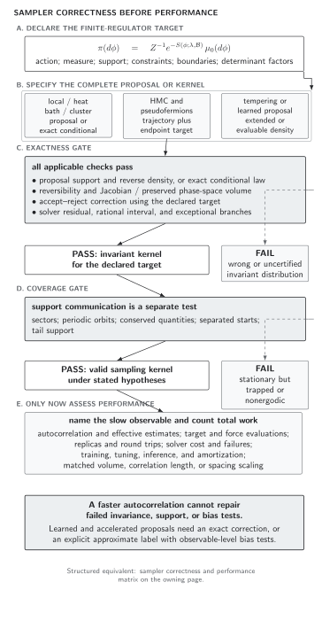
Acceleration changes proposal dynamics, not the standard of correctness. Tempering and learned moves require exact extended-target or density corrections and sector coverage; approximate methods need an explicit label and observable bias tests. Only then do autocorrelation, scaling, training, and amortization support a performance claim. Original schematic, not to scale.

The canonical sampler correctness and performance matrix is the structured cross-method comparison.

A matched acceleration experiment

For a multimodal finite scalar target, compare a local Metropolis baseline, parallel tempering, and a learned independence proposal.

1. Freeze one action, boundary condition, volume, and observable set. Include a mode label, action density, and at least one local observable.
2. Establish exact moments by enumeration or high-precision quadrature at the smallest volume. For a larger volume, require agreement among two independent exact kernels before performance comparison.
3. For tempering, record adjacent swap acceptance and complete round-trip times. For the flow, record support tests, Jacobian checks, exact-correction acceptance, and weight tails if reweighting is used.
4. Compute cost per effective estimate with the same autocorrelation convention. Charge tempering for every replica and charge the learned method for training under at least one stated amortization horizon.
5. Repeat over a sequence of barriers or correlation lengths. Fit scaling only over a justified range and show residuals; do not infer asymptotic exponents from two points.

The exactly corrected flow and tempering kernels may both pass target tests yet accelerate different observables. That is a scientific result, not a failure to find one universal ranking.

Adversarial failures

A learned support hole. Train $q_\theta$ on sector $A$ only, then observe nearly unit acceptance within $A$. Independence Metropolis cannot propose $B$, so the chain is nonergodic. Sector-separated starts and target-support probes must expose the failure.

An uncorrected approximation presented as exact. Drop the Metropolis step because validation acceptance was high. The resulting draws follow $q_\theta$, not $\pi$. Label them approximate and perform observable-level bias tests, or restore an exact correction.

A boundary change hidden as an acceleration. Compare periodic baseline data with open-boundary accelerated data without changing the finite-volume interpretation. Faster topology is real, but the two regulated targets differ. Match a common continuum observable with explicit boundary exclusions.

A cost-free training claim. Exclude training and tuning from the learned method while charging equilibration and all target evaluations to HMC. Report both one-off and amortized costs so readers can decide which deployment regime is relevant.

Observable-level validation checklist

• Identify the slow observable and hypothesized barrier before selecting an update; measure at least one comparison observable with different mode overlap.
• Prove invariance of the complete extended or corrected kernel and test communication across sectors or modes.
• Use exact small-volume moments and at least two independent kernels before interpreting a faster autocorrelation.
• Match action, boundary conditions, volume, parameter point, observable, work units, hardware, precision, and uncertainty method.
• Report scaling range, fitted form, residuals, topology or round-trip histories, and rare failures—not only a central speedup.
• For learned proposals, test support, density normalization or change of variables, Jacobians, exact correction, weight tails, training cost, and held-out transfer.
• Inject a support hole, omitted swap ratio, missing correction, or uncharged training stage and require the corresponding correctness or performance conclusion to fail.

Learning outcomes

After completing this page, you should be able to:

• diagnose a critical, topological, or multimodal slow observable and choose an acceleration whose invariant-measure argument matches that mechanism; and
• compare a baseline and accelerated method under matched targets and total costs, including exact correction, training, scaling, and observable-level failure tests.

Exercises

1. Derive the two-sector autocorrelation time. Starting from $K_p$, compute $\rho(t)$ and $\tau_{\mathrm{int}}$ for the sector indicator.

Solution

The centered sector indicator is the eigenvector $(1,-1)$ with eigenvalue $\lambda=1-2p$. Therefore $\rho(t)=\lambda^t$. Since $0<p\le1/2$, the geometric sum converges and $\tau_{\mathrm{int}}=1/2+\lambda/(1-\lambda)=(1-p)/(2p)$.

2. Prove tempering invariance. Show detailed balance for a swap of replicas $i$ and $j$ under the displayed acceptance rule.

Solution

Before the swap, the relevant extended weight is $\pi_i(x_i)\pi_j(x_j)$; afterward it is $\pi_i(x_j)\pi_j(x_i)$. The proposal to swap is its own reverse. Multiplying the old weight by the minimum of one and the ratio gives the minimum of the old and new weights, which is symmetric. All unswapped factors cancel.

References

• Abbott, R., Albergo, M. S., Botev, A., Boyda, D., Cranmer, K., Hackett, D. C., Kanwar, G., Matthews, A. G. D. G., Racanière, S., Razavi, A., Rezende, D. J., Romero-López, F., Shanahan, P. E., and Urban, J. M. (2023). “Normalizing Flows for Lattice Gauge Theory in Arbitrary Space-Time Dimension.” arXiv:2305.02402 [hep-lat]. arXiv; Open PDF.
• Albergo, M. S., Kanwar, G., and Shanahan, P. E. (2019). “Flow-based generative models for Markov chain Monte Carlo in lattice field theory.” Physical Review D 100, 034515. doi:10.1103/PhysRevD.100.034515; Open PDF.
• Kanwar, G., Albergo, M. S., Boyda, D., Cranmer, K., Hackett, D. C., Racanière, S., Rezende, D. J., and Shanahan, P. E. (2020). “Equivariant flow-based sampling for lattice gauge theory.” Physical Review Letters 125, 121601. doi:10.1103/PhysRevLett.125.121601; Open PDF.
• Lawrence, S. (2025). “Machine-learning approaches to accelerating lattice simulations.” Proceedings of Science, LATTICE2024, 010. doi:10.22323/1.466.0010; Open PDF.
• Lüscher, M., and Schaefer, S. (2011). “Lattice QCD without topology barriers.” Journal of High Energy Physics 07, 036. doi:10.1007/JHEP07(2011)036; Open PDF.
• Schaefer, S., Sommer, R., and Virotta, F. (2011). “Critical slowing down and error analysis in lattice QCD simulations.” Nuclear Physics B 845(1), 93–119. doi:10.1016/j.nuclphysb.2010.11.020; Open PDF.