Renormalizing a Truncated Hamiltonian

A truncated Hamiltonian approaches the target QFT only after omitted virtual states are represented by cutoff-dependent effective terms or shown to be negligible at the claimed accuracy. Those terms should be derived from a Feshbach–Schur reduction, short-distance expansion, or matching calculation; their coefficients must be fixed by declared inputs at every cutoff; and unused observables must test both the Hamiltonian and the associated effective operators. Fitting one energy is renormalization input, not convergence evidence.

Required background. Hilbert-Space Truncation as a Regulator supplies the $P/Q$ split. Basis Construction, Symmetry Sectors, and Matrix Elements supplies the checked finite matrices. Integrating Out Heavy Fields supplies effective-theory matching, and Regulator Removal and Renormalized Predictions supplies the continuum-limit logic.

Helpful background. Conformal and Hamiltonian Truncation supplies a UV basis whose OPE organizes high-energy tails. Operator Mixing and Renormalization Matrices supplies the operator-mixing language needed when several induced terms share quantum numbers.

Exact elimination defines the effective Hamiltonian

Renormalization and no-double-counting contract. Declare the retained projector, the operator basis in $H_{\mathrm{eff}}$, the approximation to the omitted resolvent, the subtraction convention, the observables used to fix coefficients, the refit protocol at each cutoff, and held-out tests. Every diagram, high-state sum, or perturbative term must appear exactly once: either explicitly in the retained calculation, in a computed tail, or in a matched coefficient.

With $P+Q=1$, the exact low-space equation is

$$\left[PHP+PHQ(E-QHQ)^{-1}QHP\right]|\psi_P\rangle =E|\psi_P\rangle.$$

Call the second term $\Delta H(E)$. For $H=H_0+gV$ and a projector diagonal in $H_0$, its leading perturbative form is

$$\Delta H_{ij}^{(2)}(E) =g^2\sum_{a\in Q} \frac{V_{ia}V_{aj}}{E-E_a^{(0)}}.$$

The denominator sign is physical: omitted states above the target generally lower low energies at second order. Replacing $E$ by a reference energy and expanding in $E/E_a^{(0)}$ produces energy-independent matrices plus controlled corrections only when the omitted spectrum is separated from the states of interest. Near an omitted threshold the resolvent cannot be expanded this way; the relevant states must be retained or the full energy dependence kept. This exact projection-operator reduction is the Feshbach construction Feshbach 1958, §§ 2–3.

Effective Hamiltonians that systematically approximate this tail and analyze the required counterterms are constructed in Elias Miró and Ingoldby 2023, §§ 2–5. Cohen, Farnsworth, Houtz, and Luty formulate the method as an effective field theory in which high-energy states determine local operators and power-suppressed errors Cohen et al. 2022, §§ 2–4.

Local counterterms are an expansion, not an identity

For sufficiently high omitted energies, short-time or short-distance products of the interaction can be expanded in operators allowed by the regulator’s exact symmetries:

$$\Delta H(E;\Lambda) =\sum_a c_a(\Lambda)\,\mathcal O_a^{(P)} +\Delta H_{\mathrm{nonlocal}}(E;\Lambda) +R_N(E;\Lambda).$$

The first term contains local or quasi-local projected operators; the second retains important nonlocal or energy-dependent structure; and $R_N$ is the remainder after truncating the operator expansion. Power counting and OPE data predict which $c_a$ can matter and how their leading cutoff dependence scales. Symmetry determines mixing blocks, but operators with the same quantum numbers generally mix.

State dependence is not automatically a defect. The exact $H_{\mathrm{eff}}$ is energy dependent. The defect is to replace it by a universal local Hamiltonian without estimating the induced state dependence. Conversely, fitting an independent coefficient for every eigenvalue has no predictive content.

In two-dimensional $\phi^4$ Hamiltonian truncation, explicit high-energy corrections substantially improve convergence, and next-to-leading effective Hamiltonians address residual nonlocal effects Elias-Miró, Rychkov, and Vitale 2017, §§ 2–4. These results establish the method in that declared setting; they do not prove that the same finite operator basis controls every theory or regulator.

Matching separates inputs from predictions

Write a practical finite-cutoff Hamiltonian as

$$H_\Lambda(\mathbf c) =P_\Lambda H_{\mathrm{bare}}P_\Lambda +\Delta H_{\mathrm{calc}}(\Lambda) +\sum_{a=1}^{N_c}c_a(\Lambda)\mathcal O_a^{(P)}.$$

At every $\Lambda$, determine the same $N_c$ coefficients from the same renormalization conditions

$$F_r\!\left[H_\Lambda(\mathbf c),O_{\Lambda}\right] =F_r^{\mathrm{input}}, \qquad r=1,\ldots,N_c.$$

Examples are a vacuum-energy convention, one mass gap, a scattering datum, or a matrix-element normalization. A second gap, a transition matrix element, or a quench response not appearing among the $F_r$ is a prediction. If all reported quantities are used to fit $\mathbf c$, the calculation tests only whether the parametrization can interpolate them.

The subtraction convention prevents double counting. If $\Delta H_{\mathrm{calc}}$ already includes the high-state contribution to the mass at order $g^2$, a fitted mass coefficient must represent the residual under that same convention, not add the full $g^2$ counterterm again. A useful implementation stores each contribution separately and checks $\partial H_\Lambda/\partial c_a=\mathcal O_a^{(P)}$.

Exactly checkable three-state benchmark

Let two retained states couple to one omitted state:

$$H=\begin{pmatrix} 0&0&1\\ 0&1&2\\ 1&2&10 \end{pmatrix}, \qquad P=\operatorname{diag}(1,1,0).$$

The characteristic polynomial is

$$E^3-11E^2+5E+1=0,$$

with eigenvalues, to six decimals,

$$E=(-0.149895,\ 0.634429,\ 10.515466).$$

Exact elimination of the third state gives

$$H_{\mathrm{eff}}(E) =\begin{pmatrix}0&0\\0&1\end{pmatrix} +\frac1{E-10} \begin{pmatrix}1&2\\2&4\end{pmatrix},$$

and reproduces the two low roots exactly. Expanding at $E=0$ gives

$$H_{\mathrm{eff}}^{(0)} =\begin{pmatrix}-0.1&-0.2\\-0.2&0.6\end{pmatrix},$$

whose eigenvalues are $-0.153113$ and $0.653113$. The bare projection gives $0$ and $1$. If one instead adds $cI$ and tunes $c=-0.149895$ to the exact ground energy, the excited prediction is $0.850105$, far from $0.634429$. The missing off-diagonal and relative diagonal structure is a concrete example of counterterm-basis insufficiency that a fitted ground energy cannot expose.

The convergence map makes fitting a branch, not the endpoint

In the shared map, the exact omitted-state branch produces both $H_{\mathrm{eff}}$ and $O_{\mathrm{eff}}$. Matching fixes declared inputs; held-out and cross-basis tests determine whether the chosen operator expansion is adequate.

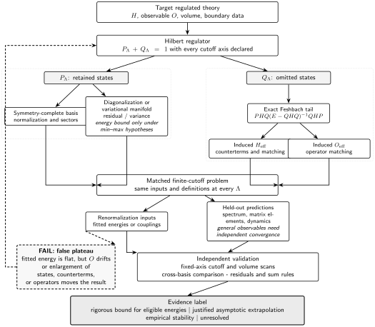
Omitted states induce correlated Hamiltonian and observable corrections. Counterterm matching fixes only the input branch; multi-cutoff residuals, held-out observables, operator-basis enlargement, and cross-basis agreement test the prediction. A fitted energy can form the schematic false plateau even when a matrix element drifts.

Minimum truncation certification record

Required fields for a truncation result and the test that can falsify each field.

Field	Required declaration	Independent test	Failure signal
Target	Hamiltonian, prior regulator, volume, boundary data, observable	Units and free or exact limit	Changing target across cutoff points
Projectors	PΛ, QΛ, all cutoff axes, limit order	State counts and nestedness	Unidentified omitted states
Basis and sectors	Normalization, Gram matrix, null removal, exact charges	Hermiticity and selection rules	Duplicates or broken constraints
Induced Hamiltonian	Derived operator basis and approximation order	Omitted-state toy model or perturbative coefficient	Drift incompatible with the declared tail
Counterterms	Inputs, running coefficients, and no-double-counting rule	Refit protocol at every cutoff	A fitted datum presented as a prediction
Variational status	Manifold, optimizer, symmetry, bound hypotheses	Residual, variance, and ansatz enlargement	Energy plateau with a large residual
Effective observables	Projected and induced operator terms	Sum rule or matched matrix element	Spectrum stable while the observable drifts
Cutoff sequence	Independent basis, volume, counterterm, time, and state scans	Fixed-axis and cross-term fits	Only one diagonal sequence
Extrapolation	Asymptotic form, fit window, covariance, alternatives	Window and model stability	Exponent chosen from the desired answer
Held-out tests	Unused spectrum, matrix element, dynamics, and second basis	Blind comparison after choices freeze	All tests participated in tuning
Adversarial enlargement	Larger state and operator bases	Repeat the full match and prediction	Former plateau moves beyond its error
Claim	Bound, asymptotic evidence, empirical stability, or unresolved	Error and cost reproduced independently	Precision exceeds the weakest test

Adversarial failure: double-counted high states

Suppose a calculation adds an analytically computed order-$g^2$ high-energy mass shift and then fits a mass counterterm formula imported from a scheme in which that same high-energy contribution was not separated. The fitted input mass can remain exact at every cutoff, hiding the duplication. A held-out gap or matrix element inherits an order-$g^2$ error and may approach a stable but wrong value.

To diagnose this failure, turn each contribution on separately, verify its perturbative coefficient against an explicit high-state sum, state the subtraction scheme, and repeat the match after enlarging the operator basis. The fitted mass is not a diagnostic because the fitting step removes its residual by construction.

Observable-level validation checklist

• Reproduce the two- and three-state Feshbach benchmarks, including the resolvent sign and energy dependence.
• Compare derived high-energy coefficients with explicit omitted-state sums in a range where both can be computed.
• Verify regulator symmetries and include every operator allowed at the claimed order; record excluded terms and their estimated size.
• Store computed tails, bare terms, fitted counterterms, and subtractions separately to expose double counting.
• Refit the same inputs at every cutoff and label them as inputs in all plots and tables.
• Test at least one unused spectral quantity and one effective-operator matrix element, then enlarge both state and operator bases.
• Repeat the prediction in a second basis and scan volume independently of the ultraviolet cutoff.

You should now be able to (1) derive the leading omitted-state Hamiltonian and classify its local, nonlocal, energy-dependent, and state-dependent pieces, and (2) define a matching scheme with an explicit subtraction rule and held-out observable. Observables and Dynamics in Truncated Spaces constructs the corresponding effective operators; Convergence, Extrapolation, and Error Certification tests their cutoff removal. General matching remains in Integrating Out Heavy Fields. Dated precision records, method rankings, and open disputes about the present reach of counterterm schemes belong to Research: Lattice and Hamiltonian Field Theory.

Exercises

Check the three-state effective Hamiltonian

Show that the determinant equation for the energy-dependent $2\times2$ $H_{\mathrm{eff}}(E)$ above reproduces the cubic characteristic polynomial of the full matrix.

Solution

Set $D=E-10$. Then

$$E-H_{\mathrm{eff}}(E) =\begin{pmatrix}E-1/D&-2/D\\-2/D&E-1-4/D\end{pmatrix}.$$

Multiplying its determinant by $D$ gives

$$D E(E-1)-4E-(E-1)=E^3-11E^2+5E+1.$$

The excluded root $E=10$ is not a pole-cancelled solution; the three roots of the cubic are precisely the full eigenvalues. The two roots away from the omitted-state pole are the intended low-space solutions.

Design a two-parameter match

A symmetry allows identity and mass operators in $H_\Lambda$. Which two conditions can fix their coefficients, and name two quantities that should remain held out.

Solution

One possible scheme fixes the vacuum energy to a declared convention and the lowest odd-sector mass gap to a physical input. At every cutoff, solve those two conditions for the identity and mass coefficients using the same subtraction convention. The first even excitation and an unfitted $\phi^2$ transition matrix element can then be held out. Other choices are valid, but two independent coefficients require two independent inputs and neither input may later be counted as a prediction.

References

• Cohen, Timothy, Kara Farnsworth, Rachel Houtz, and Markus A. Luty. “Hamiltonian Truncation Effective Theory.” SciPost Physics 13, 011 (2022). DOI. Open PDF.
• Elias Miró, Joan, and James Ingoldby. “Effective Hamiltonians and Counterterms for Hamiltonian Truncation.” Journal of High Energy Physics 2023, 052 (2023). DOI. Open PDF.
• Elias Miró, Joan, Slava Rychkov, and Lorenzo G. Vitale. “NLO Renormalization in the Hamiltonian Truncation.” Physical Review D 96, 065024 (2017). DOI.
• Feshbach, Herman. “Unified Theory of Nuclear Reactions.” Annals of Physics 5, no. 4 (1958): 357–390. DOI.