Autocorrelation Times and Effective Sample Size

Successive configurations in a Markov chain are correlated. The variance of a sample mean is therefore controlled by an observable-specific integrated autocorrelation time, not by the stored configuration count alone. Estimating that time requires a finite lag window, a slow-tail assessment, and uncertainty on the estimate itself.

Required background. Markov-chain sampling defines the stationary history and update unit.

Helpful background. Markov generators, ergodicity, and sampling error explain spectral slow modes.

Autocorrelation functions and conventions

Local statistical convention and regime. The history is an ordered, post-cut stationary stream indexed by one declared update unit; rejected configurations remain repeated entries. Autocorrelation times use $\tau_{\mathrm{int}}=\tfrac12+\sum_{k\ge1}\rho(k)$ and are first reported in stored-measurement units, then converted to elementary updates or trajectories. Every estimate retains the finite window, any tail model, stream boundaries, and uncertainty on $\widehat\tau_{\mathrm{int}}$.

For a stationary scalar history $X_t$ with mean $\mu$, define

$$\Gamma_X(k)=\langle(X_t-\mu)(X_{t+k}-\mu)\rangle, \qquad \rho_X(k)=\frac{\Gamma_X(k)}{\Gamma_X(0)}.$$

This page uses

$$\tau_{\mathrm{int},X}=\frac12+\sum_{k=1}^{\infty}\rho_X(k).$$

For $N$ consecutive measurements much longer than the slowest relevant time,

$$\operatorname{var}(\overline X)\simeq \frac{2\tau_{\mathrm{int},X}}{N}\Gamma_X(0), \qquad N_{\mathrm{eff},X}=\frac{N}{2\tau_{\mathrm{int},X}}.$$

Some literature defines $1+2\sum\rho$ as the autocorrelation time. State the convention before comparing numbers; Sokal 1997, pp. 131–192 uses the correlation-aware variance framework and makes this normalization dependence explicit.

The exponential time $\tau_{\exp}$ describes the slowest mode with nonzero overlap, $\rho(k)\sim Ae^{-k/\tau_{\exp}}$. An observable with small amplitude $A$ can have modest $\tau_{\mathrm{int}}$ while still carrying a long tail that matters at high precision.

The exactly soluble AR(1) benchmark

For

$$X_t=\rho X_{t-1}+\sqrt{1-\rho^2}\,\epsilon_t, \qquad \epsilon_t\sim N(0,1),$$

the stationary variance is one and $\rho_X(k)=\rho^k$. Hence

$$\tau_{\mathrm{int}}=\frac12+\frac{\rho}{1-\rho} =\frac{1+\rho}{2(1-\rho)}.$$

At $\rho=0.8$, $\tau_{\mathrm{int}}=4.5$ and $N_{\mathrm{eff}}=N/9$. This fixture tests normalization, lag indexing, window selection, and coverage of the reported mean.

Windowing and slow tails

The direct estimator truncates the noisy sum at $W$:

$$\widehat\tau_{\mathrm{int}}(W)=\frac12+ \sum_{k=1}^{W}\widehat\rho(k).$$

Small $W$ biases downward by omitting positive tails; large $W$ accumulates noisy sample correlations. A self-consistent window such as $W\approx c\widehat\tau_{\mathrm{int}}(W)$ balances these effects, but $c$ and the stopping rule must be stated. Plot stability versus $W$ and compare replicas or longer chains. The bias–variance tradeoff and automatic-window logic are developed in Madras and Sokal 1988 and Wolff 2004, pp. 143–153.

If a theoretically motivated slow observable or mode has decay time $\tau_s$ and amplitude estimate $A_s$, a tail correction can bound

$$\sum_{k>W}\rho(k)\approx A_s\frac{e^{-(W+1)/\tau_s}}{1-e^{-1/\tau_s}}.$$

This is a model-dependent bound, not measured information. Report it separately and vary the tail assumptions.

The dependency graph shows why this choice propagates into every downstream covariance and fit.

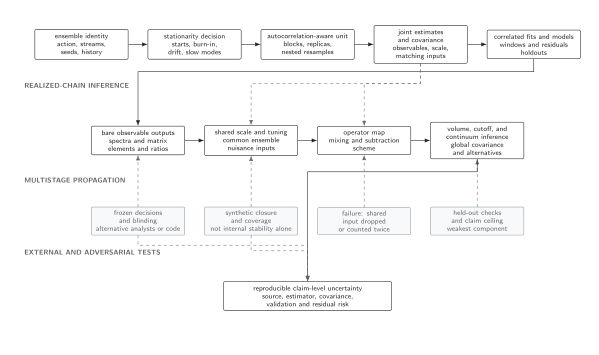
The autocorrelation window determines the effective information entering all later stages. Shared configurations and nuisance inputs remain correlated through resampling, fitting, and extrapolation. The diagram is schematic.

Observable dependence and derived quantities

Different observables overlap differently with slow transition-kernel modes. Report $\tau_{\mathrm{int}}$ for the target observable, scale setter, topological charge, and any important fit direction. For a vector $\mathbf X$, the relevant slow combination for $f(\overline{\mathbf X})$ is approximately $\nabla f^T\mathbf X$; separate component times can miss cancellation or amplification.

Measurement spacing changes units but not independent information. If every $s$th update is stored, $\tau$ in stored samples may shrink roughly by $s$, while the cost per effective sample should be quoted in elementary updates or wall-clock work.

Adversarial failure: a weak slow mode hidden by a fast monitor

A sum of two independent stationary AR(1) processes can have the exactly normalized correlation

$$\rho(k)=0.99(0.5)^k+0.01(0.995)^k.$$

The first few lags appear fast, yet

$$\tau_{\mathrm{int}} =\frac12+0.99\frac{0.5}{1-0.5} +0.01\frac{0.995}{1-0.995} =3.48.$$

Truncating at $W=10$ gives only $\widehat\tau_{\mathrm{int}}=1.586\ldots$, missing more than half the variance inflation even though the slow mode has amplitude $0.01$. An implementation must recover the analytic value as chains lengthen and must fail a precision claim when its window rule cannot resolve or bound this injected tail.

Observable-level validation checklist

• Preserve configuration order, rejected states, stream boundaries, and the conversion between stored measurements and elementary updates.
• Plot $\widehat\rho_X(k)$ and the window scan for the target observable, scale setter, sector-sensitive observable, and important derived direction.
• Recover $\tau_{\mathrm{int}}=(1+\rho)/[2(1-\rho)]$ and nominal mean coverage on repeated AR(1) histories.
• Inject the two-mode adversary above and verify that a tail study, longer replica, or declared bound prevents the $W=10$ underestimate from passing.
• Vary measurement spacing and confirm that $N_{\mathrm{eff}}$ expressed per elementary update is unchanged within uncertainty.
• Report $\widehat\tau_{\mathrm{int}}$, its uncertainty, the chosen window and tail rule, $N_{\mathrm{eff}}$, and cost per effective sample for each material observable.

Common pitfalls

Using the chain length as the sample size. The effective count can be orders of magnitude smaller and differs by observable.

Stopping the sum at the first negative estimate. Noise can create an early sign change and severe downward bias. Use a declared window and stability study.

Diagnosing only a fast observable. Energy or plaquette histories can look healthy while topology or long-distance modes remain frozen.

Learning outcomes

1. Given repeated AR(1) or two-mode synthetic histories, estimate $\tau_{\mathrm{int}}$ with a stated window and demonstrate bias, variance, and interval coverage against the analytic value.
2. Given target and slow-control histories, report observable-specific $N_{\mathrm{eff}}$ in update units and reject a naive independent-sample error when an unresolved tail changes the uncertainty materially.

Exercises

1. For $N=9000$ and AR(1) $\rho=0.8$, compute $N_{\mathrm{eff}}$.

Solution

$2\tau_{\mathrm{int}}=9$, so $N_{\mathrm{eff}}=1000$.

2. If configurations are stored every four updates, what happens to the unit of $\tau_{\mathrm{int}}$?

Solution

The numerical time is then measured in stored-configuration intervals. Convert back by multiplying by four for update units; thinning does not create additional independent information.

References

• Madras, N., and Sokal, A. D. (1988). The pivot algorithm: a highly efficient Monte Carlo method for the self-avoiding walk. Journal of Statistical Physics, 50, 109–186. DOI.
• Sokal, A. D. (1997). Monte Carlo methods in statistical mechanics: foundations and new algorithms. In C. DeWitt-Morette, P. Cartier, and A. Folacci (eds.), Functional Integration: Basics and Applications, pp. 131–192. Springer New York. DOI.
• Wolff, U. (2004). Monte Carlo errors with less errors. Computer Physics Communications, 156, 143–153. DOI.