Anatomy and Severity of a Sign Problem

A sign problem occurs when the exact weight cannot be used as a nonnegative probability measure in the chosen representation. Its practical severity is not one number: phase cancellation controls the denominator of reweighting, overlap controls whether important target configurations are sampled, and correctness controls whether a replacement process computes the intended integral. Confusing these mechanisms produces confident but invalid error estimates.

Required background. Chemical potential on the Euclidean lattice supplies the complex determinant and charge convention.

Helpful background. Probability, random variables, and conditional expectation supplies variance and importance sampling. Complete lattice error budgets supplies the distinction between statistical and method bias.

Phase quenching and exact reweighting

Convention and regulator card. Work at finite lattice spacing and finite spatial volume $V_s$, with inverse temperature $\beta_T$. Write the regulated weight as $w(x)=|w(x)|e^{i\phi(x)}$ and assume $Z_{\rm pq}=\int dx\,|w(x)|$ is finite and nonzero. The subscript “pq” means this precisely defined phase-quenched measure; it is not automatically the same physical theory with one parameter changed.

For any integrable observable,

$$\langle O\rangle =\frac{\int dx\,|w|e^{i\phi}O}{\int dx\,|w|e^{i\phi}} =\frac{\langle Oe^{i\phi}\rangle_{\rm pq}} {\langle e^{i\phi}\rangle_{\rm pq}}.$$

The average phase is a partition-function ratio,

$$m\equiv\langle e^{i\phi}\rangle_{\rm pq} =\frac{Z}{Z_{\rm pq}}.$$

When the two ensembles admit thermodynamic free-energy densities $f$ and $f_{\rm pq}$,

$$|m|=\exp[-\beta_TV_s\Delta f+o(V_s)], \qquad \Delta f=\operatorname{Re}f-f_{\rm pq}\ge0.$$

The inequality follows from $|Z|\le Z_{\rm pq}$. The statement is asymptotic and representation dependent because $Z_{\rm pq}$ changes when the decomposition into magnitude and phase changes.

What the average phase predicts

For $N$ independent phase samples $u_k=e^{i\phi_k}$, the sample mean $\bar u$ has

$$\mathbb E|\bar u-m|^2=\frac{1-|m|^2}{N}.$$

Its relative mean-square error is therefore

$$\frac{\mathbb E|\bar u-m|^2}{|m|^2} =\frac{1-|m|^2}{N|m|^2}.$$

If $|m|\sim e^{-\beta_TV_s\Delta f}$, keeping this relative error fixed requires $N\sim e^{2\beta_TV_s\Delta f}$ independent samples. Autocorrelation multiplies the cost through the integrated autocorrelation time. Ratio observables can be better or worse depending on covariance between numerator and denominator, so the phase-only estimate is a severity baseline, not a universal error bar.

The figure separates this cancellation law from overlap, ordinary instability, and worst-case complexity. Inspect the arrows: they share a complex measure, but none is logically interchangeable with another.

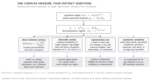
The sign problem has distinct diagnostics. The average phase fixes direct phase-estimator signal-to-noise and may scale as $e^{-\beta_TV_s\Delta f}$; overlap depends on the target observable and proposal measure; a variable change can trade phase for nonlocality or hard observables; and worst-case complexity requires a separately specified problem family. The map is schematic, not a quantitative performance comparison.

Overlap is observable dependent

Let $p(x)$ be the proposal distribution and let $A$ be a region important for the target numerator. If $p(A)=\varepsilon\ll1$, then the probability of seeing no sample in $A$ after $N$ independent draws is

$$(1-\varepsilon)^N\simeq e^{-N\varepsilon}.$$

Thus $N\gg1/\varepsilon$ is necessary even before phase cancellation is considered. A useful diagnostic is the distribution of log-weight differences, not merely the mean phase. For positive importance weights $r=p_*/p$, the population effective fraction

$$\frac{N_{\rm eff}}{N}≈ \frac{(\mathbb E_p r)^2}{\mathbb E_p r^2} =e^{-D_2(p_*\Vert p)}$$

is governed by a Rényi divergence when the moments exist. Complex weights do not define a unique effective sample size; one should report a phase statistic and a separate magnitude/overlap statistic.

An observable can be supported in a tail invisible to a global average phase. Conversely, a small average phase need not make every symmetry-protected ratio impossible if numerator and denominator correlations are exploited with a justified estimator. The reliability question is always: which configurations dominate this observable, and how were they sampled?

Exact independent-copy benchmark

Use the one-angle weight

$$w(\theta;\mu)=e^{\cos\theta} \bigl(1+0.2e^{\mu+i\theta}\bigr) \bigl(1+0.2e^{-\mu-i\theta}\bigr)$$

and define $z=\int_{-\pi}^{\pi}w\,d\theta$, $z_{\rm pq}=\int_{-\pi}^{\pi}|w|\,d\theta$, and $r=z/z_{\rm pq}$. For $V$ independent copies,

$$Z_V=z^V, \qquad Z_{{\rm pq},V}=z_{\rm pq}^V, \qquad \langle e^{i\Phi}\rangle_{{\rm pq},V}=r^V.$$

This is an exact demonstration of exponential suppression: $-V^{-1}\log|\langle e^{i\Phi}\rangle|=-\log r$. Direct quadrature of $z_{\rm pq}$ and the Bessel-function formula for $z$ are independent calculations. At imaginary $μ=i\mu_I$ with $h=0.2$, the bracket is $1.04+0.4\cos(\theta+\mu_I)>0$, so $r=1$; continuation can still fail outside its analytic domain even though sampling at the imaginary points is sign-free.

At the prescribed real points, direct quadrature gives $r(0)=1$, $r(0.5)=0.99301849$, $r(1)=0.96823563$, and $r(1.5)=0.91485248$. Raising the last value to the independent-copy volumes gives $r^{4}=0.70049$, $r^{16}=0.24078$, and $r^{64}=0.0033610$. These numbers reproduce the severity measure without fitting a free-energy slope; a Monte Carlo implementation should recover both the one-copy ratios and their exact powers.

To expose overlap independently, estimate

$$O_c(\theta)=\mathbf 1_{|\theta-\pi|<0.05}$$

under a proposal concentrated near $θ=0$. A sampler can reproduce $z$ and its average phase while never visiting the support of $O_c$. This deliberate failure distinguishes partition-function cancellation from an observable-specific rare event.

Sign, variance, overlap, and correctness

Use the following classification before choosing a method.

• Negative or complex weight: the integrand is not a probability in the selected variables. This is an algebraic property of the representation.
• Cancellation severity: $|m|$, its volume slope, cumulants of $φ$, and the covariance of the actual ratio estimator quantify statistical loss in reweighting.
• Overlap failure: important target regions are rare or absent in the proposal ensemble. Tail probabilities, weight distributions, sector occupancy, and forward/reverse comparisons diagnose it.
• Ordinary numerical instability: overflow, ill-conditioned linear solves, long autocorrelation, and optimizer failure can occur with positive weights. These require numerical remedies, not sign-problem rhetoric.
• Correctness failure: a complex stochastic or contour method converges to the wrong integral because an integration-by-parts boundary term, missing sector, Jacobian, or reconstruction tail was omitted. More samples do not remove this bias. A worst-case computational obstruction is a further, hypothesis-dependent statement, as the explicit reduction of Troyer and Wiese 2005 illustrates.

Adversarial failures

A tiny error bar around zero phase. Suppose all samples come from one phase mode and give a precise $\bar u$. If a second mode with exponentially small proposal probability contributes comparably to $Z$, the quoted variance is conditional on the wrong support. Multiple starts, sector-resolved weights, and an exact small-volume result are required.

A stable result from a modified measure. Clipping large reweighting factors, discarding configurations near determinant zeros, or replacing a complex Jacobian by its magnitude may stabilize estimates. Each operation changes the target unless its correction is included and controlled.

Exponential fit from too little range. A straight line in $-\log|m|$ over two volumes does not establish an asymptotic free-energy difference. Add volumes, check finite-size terms, and compare at fixed physical temperature and parameters.

Observable-level validation checklist

• Report the exact phase-quenched measure, $|m|$, its uncertainty, autocorrelation, and volume dependence.
• For the actual observable, inspect numerator–denominator covariance, reweighting-factor tails, sector occupancy, and at least one overlap stress test.
• Compare an exact or sign-free limit and a deliberately hostile observable or parameter point.
• Separate statistical variance, autocorrelation, overlap bias, truncation, and method-correctness uncertainty.
• Repeat the analysis after a legitimate representation change; changed severity is expected, while the exact observable must agree.

Exercises

1. Cost exponent

Assume $|m|=e^{-cV}$ and independent unit-modulus phase samples. How must $N$ scale to keep the relative root-mean-square error of $\bar u$ below $ε$?

Solution

The squared relative error is $(1-|m|^2)/(N|m|^2)$. Hence

$$N\ge\frac{1-e^{-2cV}}{\epsilon^2e^{-2cV}} =\epsilon^{-2}(e^{2cV}-1).$$

For large $V$, $N\sim\epsilon^{-2}e^{2cV}$. Correlation replaces $N$ by the number of effectively independent samples.

2. A missed rare region

A proposal assigns probability $10^{-5}$ to the region that supplies half of an observable’s numerator. How many independent samples are needed for at least 95% probability of visiting it once?

Solution

Require $1-(1-10^{-5})^N\ge0.95$. Thus

$$N\ge\frac{\log0.05}{\log(1-10^{-5})}\simeq2.996\times10^5.$$

One visit is not enough for a precise contribution; this is only a necessary support test.

Learning outcomes

After working this page, you should be able to:

• Derive the relative variance of the average-phase estimator and extract its measured volume-cost exponent with autocorrelation included.
• Given sampling evidence for an observable, classify the limiting failure as cancellation, overlap, ordinary numerical instability, or correctness bias and name a discriminating test.

Handoff

Basis dependence and computational complexity asks which of these diagnostics survive a representation change. The method pages then replace the generic warning with explicit correctness contracts.

References

• Troyer, Matthias, and Uwe-Jens Wiese. “Computational Complexity and Fundamental Limitations to Fermionic Quantum Monte Carlo Simulations.” Physical Review Letters 94 (2005): 170201. doi:10.1103/PhysRevLett.94.170201.

References

Section titled “References”- Agapiou, Sergios, Omiros Papaspiliopoulos, Daniel Sanz-Alonso, and Andrew M. Stuart. “Importance Sampling: Intrinsic Dimension and Computational Cost.” Statistical Science 32 (2017): 405–431. doi:10.1214/17-STS611.
- Alexandru, Andrei, Gökçe Başar, Paulo F. Bedaque, and Neill C. Warrington. “Complex Paths around the Sign Problem.” Reviews of Modern Physics 94 (2022): 015006. doi:10.1103/RevModPhys.94.015006.
- Elvira, Víctor, Luca Martino, and Christian P. Robert. “Rethinking the Effective Sample Size.” International Statistical Review 90 (2022): 525–550. doi:10.1111/insr.12500.
- Gattringer, Christof, and Kurt Langfeld. “Approaches to the Sign Problem in Lattice Field Theory.” International Journal of Modern Physics A 31 (2016): 1643007. doi:10.1142/S0217751X16430077. Open PDF: arXiv:1603.09517.